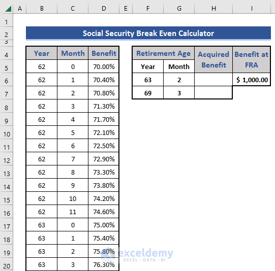
Method 1 – Insert Primary Information
- Insert basic information to compare two ages and 100% benefits in the dataset.
Method 2 – Calculate the Total Months
- Insert two new rows to calculate the total months in the dataset.
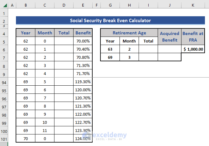
- Go to cell D5 and put in the following formula.
=$B5*12+$C5
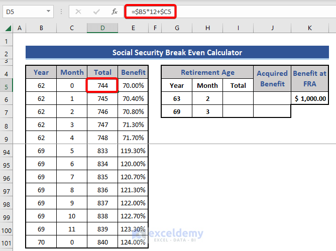
This will help you find the benefit percentage based on the age at which you took retirement. Expand this formula to the end.
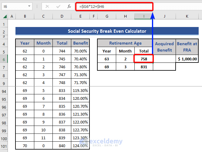
- Put another formula for cell I6 and I7.
=$G6*12+$H6
Method 3 – Find out Benefit Percentage
Use the VLOOKUP function to calculate the benefit percentage at different retirement ages.
- Put the following formula on cells J6 and J7.
For cell J6:
=VLOOKUP($I6,$D$5:$E$101,2,FALSE)
For cell J7:
=VLOOKUP($I7,$D$5:$E$101,2,FALSE)
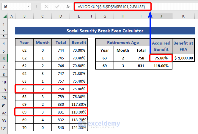
We successfully find out the percentage from the list at different retirement ages.
Method 4 – Calculate Cumulative Social Security Benefit
Here, the 1st retirement age is 63 years and 2 months. The person will benefit in the next month, which is 63 years and 3 months. After that, this will continue for a lifetime.
- Apply a formula on cell O6 to get the cumulative benefit for the 1st retirement age.
=IF($I$6<=($M5*12+$N5),$K$6*$J$6+$O5,0)
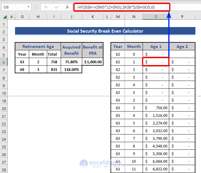
Expand this formula to the last. We used the IF function in this formula.
- Use another similar formula on cell P6 for the cumulative benefit at 2nd retirement age.
=IF($I$7<=($M5*12+$N5),$K$6*$J$7+$P5,0)
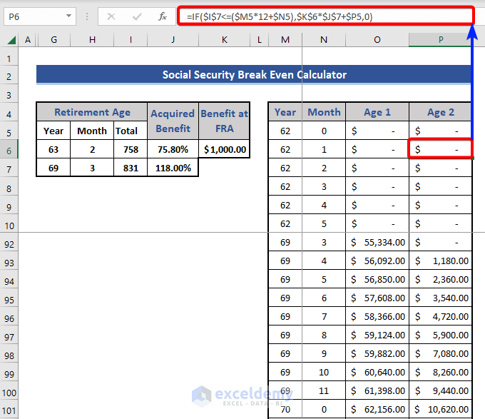
Expand this to the last cell.
Method 5 – Insert Data in a Chart to Find the Break-Even Point
- Add a new column named Level for year-defining value.
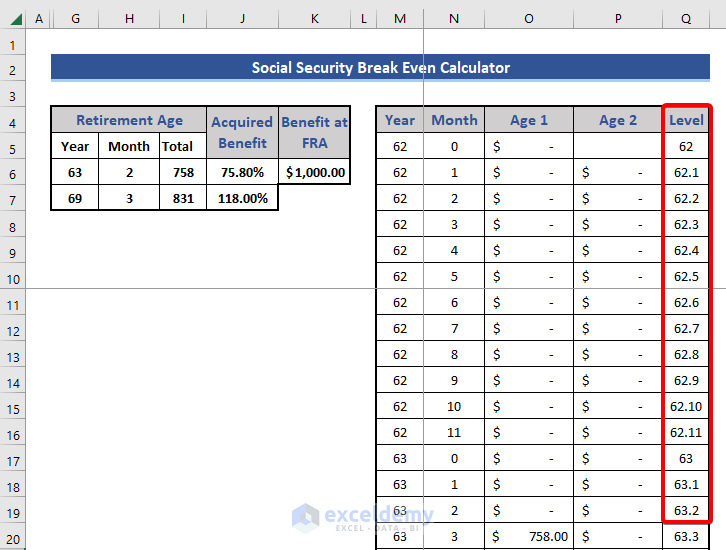
- Select the whole data from the three columns Age 1, Age 2, and Level.
- Go to the Insert tab.
- Choose the Line option from the Charts group.
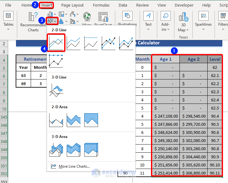
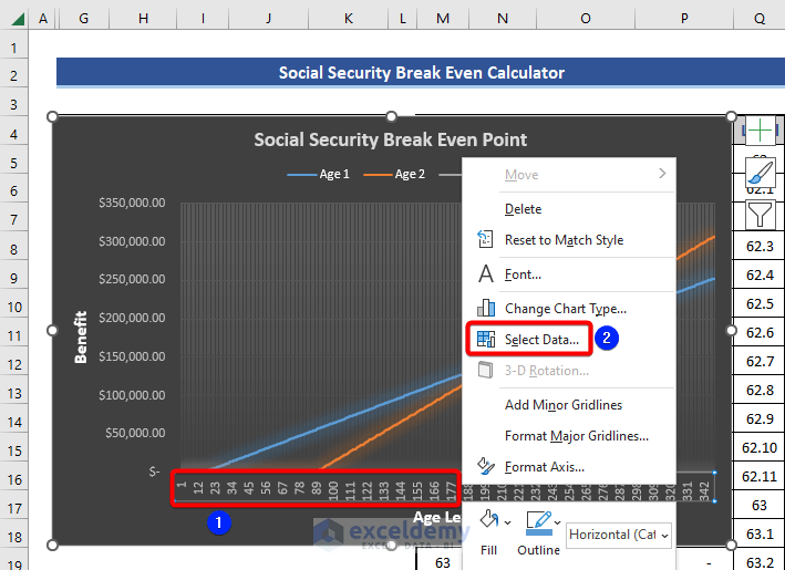
- Look at the following chart. Here, we will change the data of the horizontal axis.
- Choose the horizontal axis and press the right button of the mouse.
- Click the Select Data option from the menu.
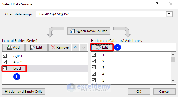
- Select Data Source window appears.
- Choose the Level option from the Legend Entries section.
- Choose the Edit option from the Horizontal Axis Labels section.
- Choose the Level column as the Axis label range.
- Press the OK button.
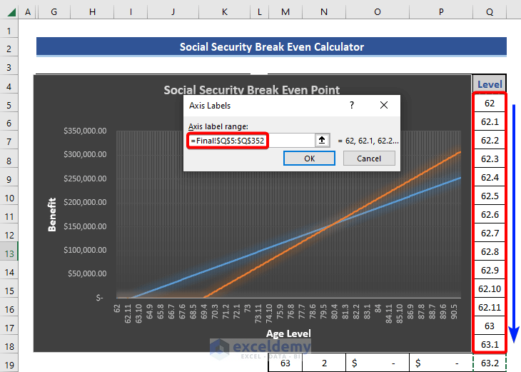
- Look at the chart now.
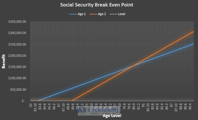
The chart will give us an idea of the break-even point, but we have to find it manually from the chart or the dataset.
Method 6 – Find Out the Break-Even Point
- Add a new column in the dataset. Put a formula on cell R5.
=IF(IF(AND(O5<>0,P5<>0),O5-P5,"N/A")<>"N/A",ABS(O5-P5),"N/A")
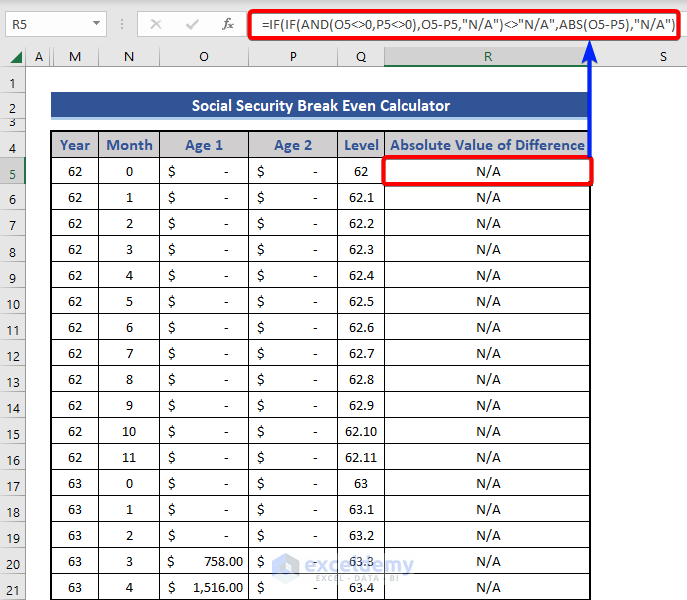
This formula uses the nested IF function to find the absolute values of the difference between the benefits of age 1 and age 2. We added a condition that when Age 1 and Age 2 are both 0, the subtraction formula will not be applied.
Formula Breakdown:
- AND(O5<>0,P5<>0)
It follows two conditions. Check if O5 and P5 are not equal to 0.
Result: False.
- IF(AND(O5<>0,P5<>0),O5-P5,”N/A”)
IF function returns the difference between O5 and P5 when fulfilling the condition. Otherwise returns “N/A”
Result: N/A.
- IF(IF(AND(O5<>0,P5<>0),O5-P5,”N/A”)<>”N/A”,ABS(O5-P5),”N/A”)
IF function works based on the value of the previous section. If the value of the previous section is not equal to N/A, give the absolute value of the difference between cell O5 and P5, Otherwise, return N/A.
Result: N/A.
- Add a section in the dataset to find out the break-even point.
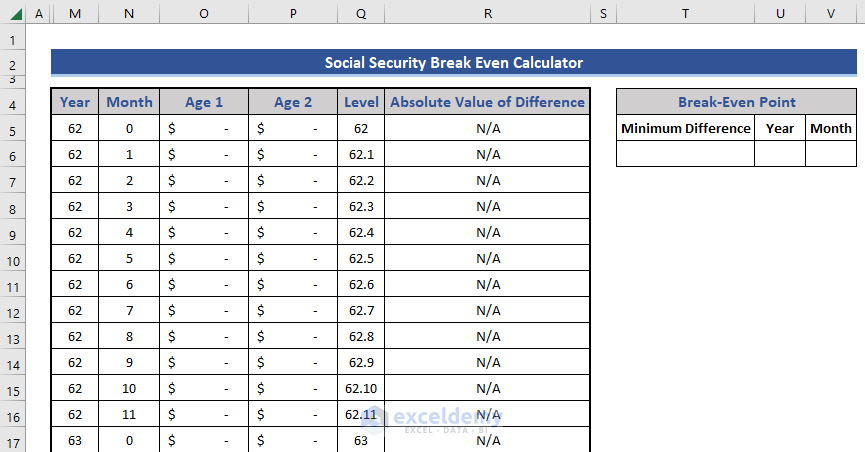
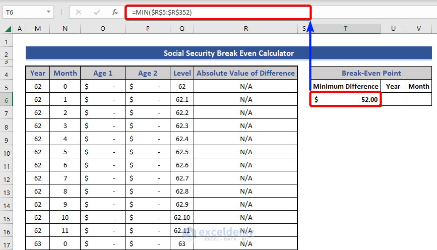
- Use the following formula based on the MIN function to get the minimum difference at cell T6.
=MIN($R$5:$R$352)
=INDEX($M$5:$M$352,MATCH($T$6,$R$5:$R$352,0))
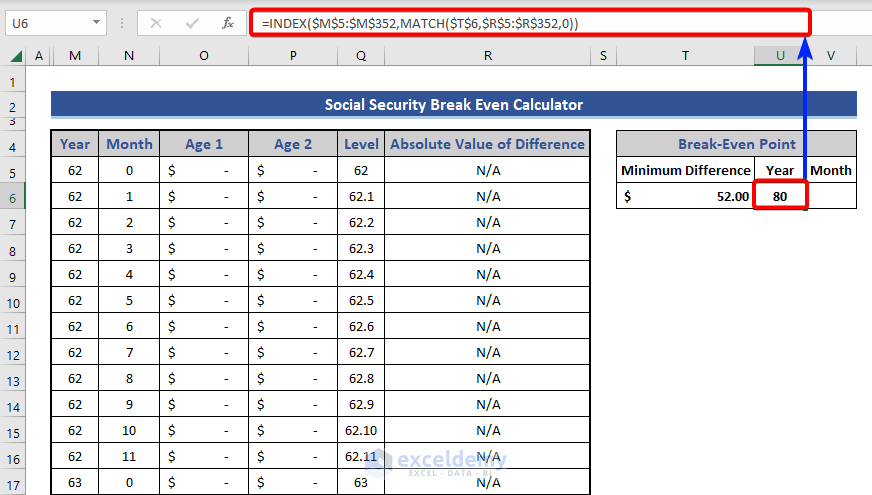
This returns the Year value. The INDEX-MATCH formula works based on the minimum difference between two ages.
- Find out the Month value.
=INDEX($N$5:$N$352,MATCH($T$6,$R$5:$R$352,0))
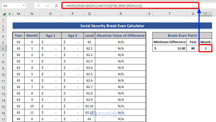
Get the break-even point at age 80 years and 2 months.
Download Practice Workbook
Download this practice workbook to exercise while you are reading this article.
<< Go Back to Break-Even Analysis | Finance Template | Excel Templates
Get FREE Advanced Excel Exercises with Solutions!

