To separate odd and even numbers:
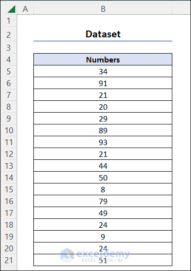
Method 1 – Combining the FILTER and the MOD Functions to Separate Odd and Even Numbers
Steps:
- In C5, enter the following formula.
=FILTER($B$5:$B$21,MOD($B$5:$B$21,2)=1)- Press Enter to see the odd numbers.
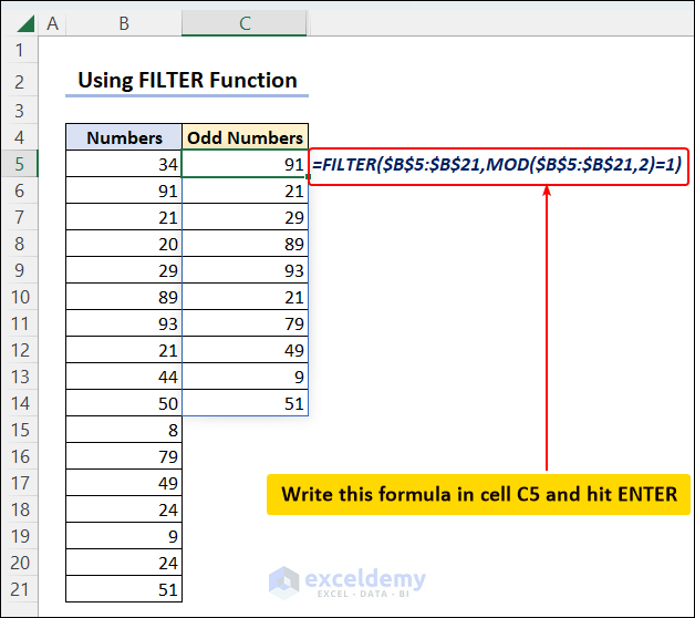
Formula Explanation:
- MOD($B$5:$B$21,2)
The MOD function returns the remainder after the numbers in B5:B21 are divided by 2.
Output: {0;1;1;0;1;1;1;1;0;0;0;1;1;0;1;0;1}
- MOD($B$5:$B$21,2)=1
This checks whether the condition set is TRUE. If it’s not TRUE, it returns FALSE.
Output: {FALSE;TRUE;TRUE;FALSE;TRUE;TRUE;TRUE;TRUE;FALSE;FALSE;FALSE;TRUE;TRUE;FALSE;TRUE;FALSE;TRUE}
- FILTER($B$5:$B$21,MOD($B$5:$B$21,2)=1)
The FILTER function returns the value from B5:B21 when it finds the condition TRUE.
Output: {91;21;29;89;93;21;79;49;9;51}
- For even numbers, the formula is:
=FILTER($B$5:$B$21,MOD($B$5:$B$21,2)=0)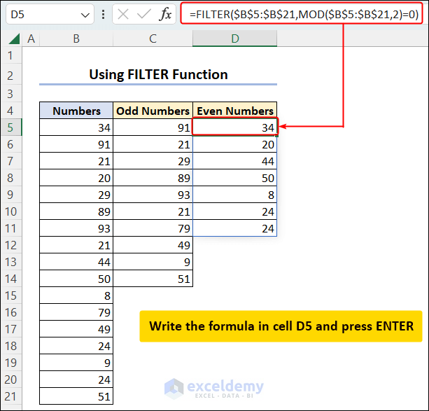
Method 2 – Use an INDEX Formula If the FILTER Function Is Not Available
Steps:
- In C5, enter the following formula to get the odd numbers.
=IFERROR(INDEX($B$5:$B$21,SMALL(IF(ISODD($B$5:$B$21+0),ROW($B$5:$B$21)),ROWS($C$5:C5))-ROW($B$4)),"")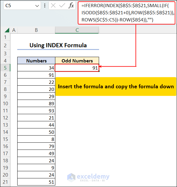
- Drag down the Fill Handle to see the result in the rest of the cells.
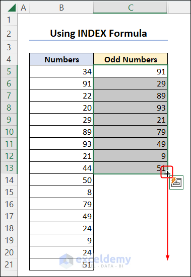
Formula Explanation:
The ISODD function will return TRUE for odd numbers (or FALSE for even numbers) to the IF function. The IF function will return the row number in B5:B21 in which the condition is TRUE. The SMALL function will find the smallest number in this array and the INDEX function will return numbers accordingly.
- The formula for even numbers is:
=IFERROR(INDEX($B$5:$B$21,SMALL(IF(ISEVEN($B$5:$B$21+0),ROW($B$5:$B$21)),ROWS($C$5:C5))-ROW($B$4)),"")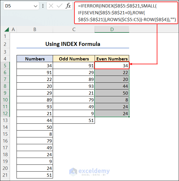
Method 3 – Separate Odd and Even Numbers in Excel by Sorting them
Steps:
- Add a helper column: column C.
- In C5, enter the following formula.
=MOD(B5,2)- Drag down the Fill Handle to see the result in the rest of the cells.
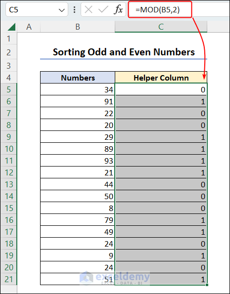
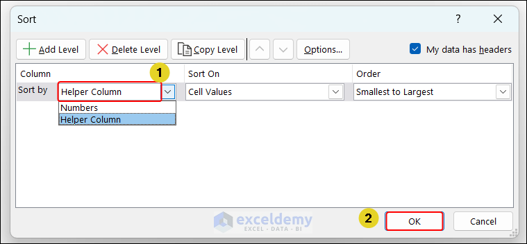
- Select B5:C21 and go to the Data tab ⇒ Sort & Filter ⇒ Sort command.
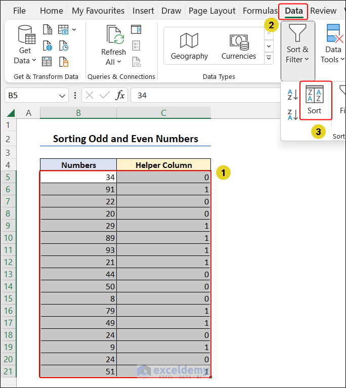
- Select Sort by: Helper Column and click OK.
The even numbers are sorted at the top and the odd numbers are at the bottom.
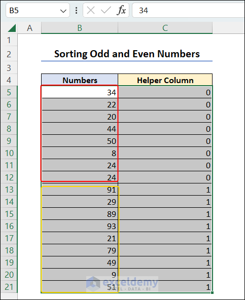
- Delete the helper column.
Method 4 – Use the IF Formula to Mark Even and Odd Numbers Separately
- In C5, enter the following formula.
=IF(ISODD(B5:B21+0),"ODD!","EVEN")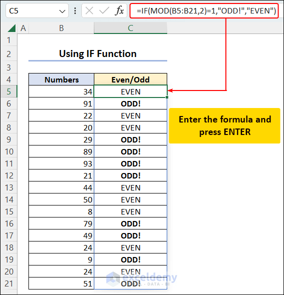
Similar Formula with MOD Function:
=IF(MOD(B5:B21,2)=1,"ODD!","EVEN")Method 5 – Filter Odd and Even Numbers in Excel
Steps:
- Add a helper column: column C.
- In C5, enter the following formula.
=ISEVEN(B5)- Drag down the Fill Handle to see the result in the rest of the cells.
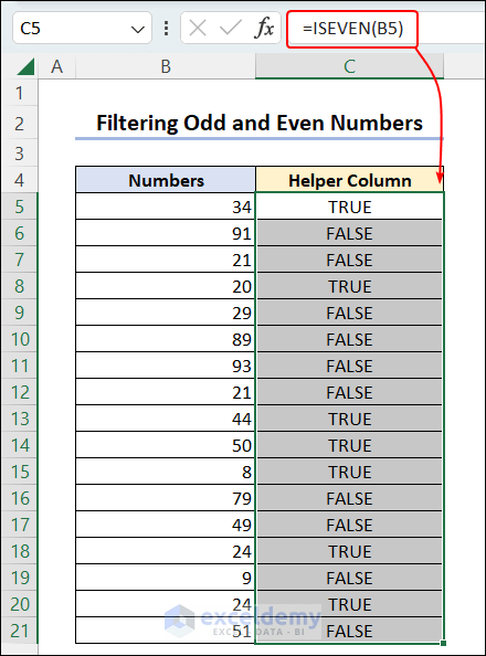
- Select a cell and go to Home ⇒ Editing ⇒ Sort & Filter ⇒ Filter.
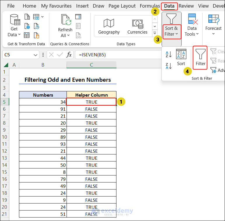
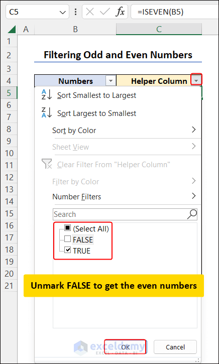
- Uncheck FALSE to get the even numbers and uncheck TRUE to get the odd numbers.
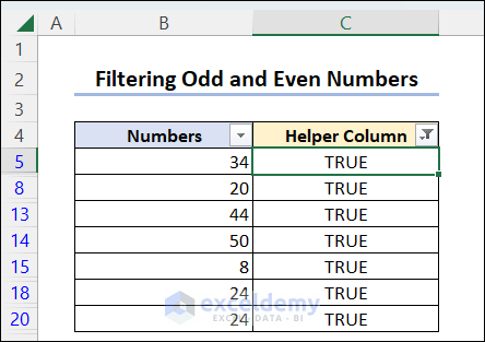
- Click OK.
Method 6 – Distinguish Odd and Even Numbers with Different Colors Using Conditional Formatting
Steps:
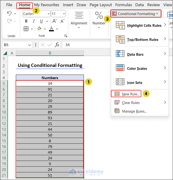
- Select B5:B21 and go to Home ⇒ Conditional Formatting ⇒ New Rule.
- Select “Use a formula to determine which cells to format” and use the following formula in Rule Description.
=ISEVEN($B5)- Click Format.
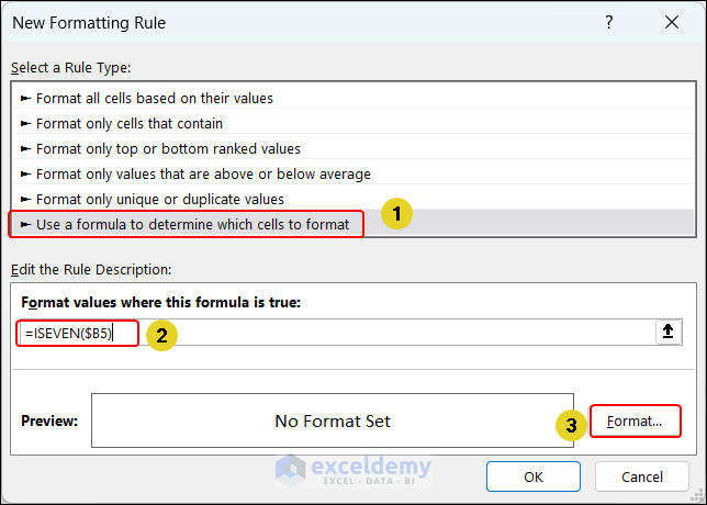
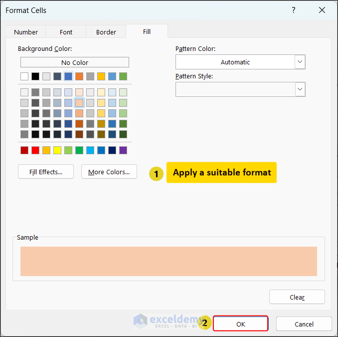
- Choose a format and click OK twice.
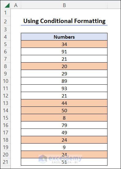
Even and odd numbers are now colored and can be distinguished.
Download Practice Workbook
Download the workbook to practice.
<< Go Back to | Excel for Math | Learn Excel
Get FREE Advanced Excel Exercises with Solutions!

