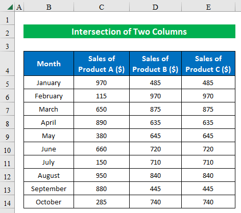
Below is a monthly sales dataset of Products A, B, and C. Using simple tricks, we will find the intersection between these sales columns.
Method 1 – Using a Combination of IF, ISERROR, and MATCH Functions
Steps:
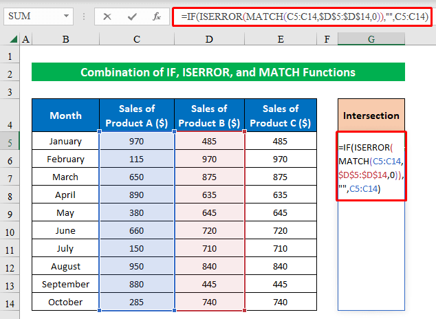
- Choose a cell (G5) and apply the below formula:
=IF(ISERROR(MATCH(C5:C14,$D$5:$D$14,0)),"",C5:C14)Where,
- The MATCH function will look for values in the lookup array ($D$5:$D$14).
- The ISERROR function will check whether the value is an error or not and return TRUE or FALSE.
- The IF function will provide the final output, checking whether the given condition is met and returning the value if it’s TRUE.
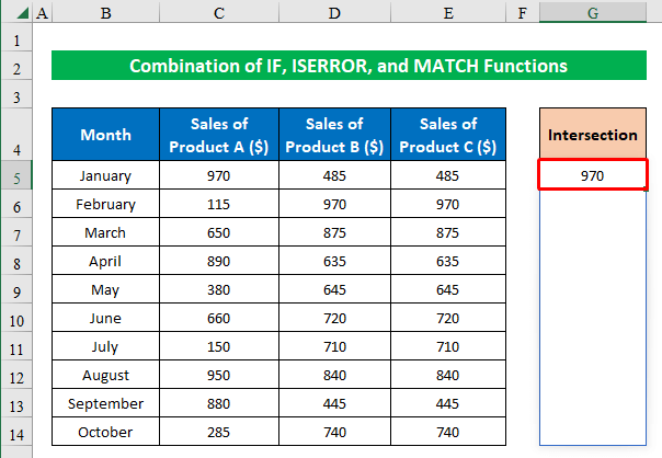
- Press ENTER.
- As a result, you will find the intersection output in the new cell.
Read More: Performing Intersection of Two Data Sets in Excel
Method 2 – Using a Space Between Column Ranges to Find Intersection of Two Columns
Steps:
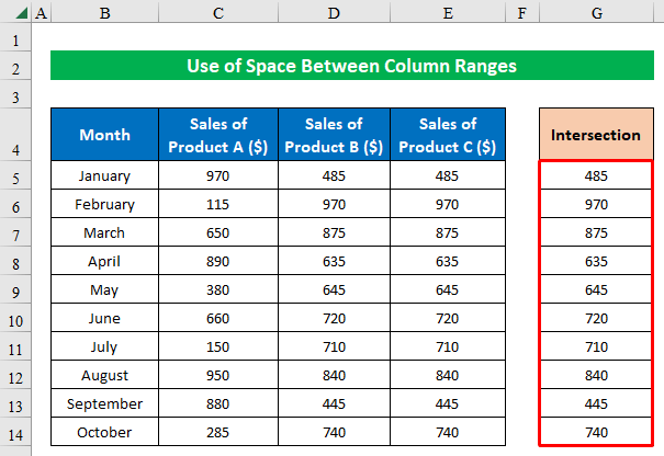
- Choose a cell (G5) and write the below formula:
=C5:D14 D5:E14Where,
- We have used a single space as an intersection operator between two column ranges.
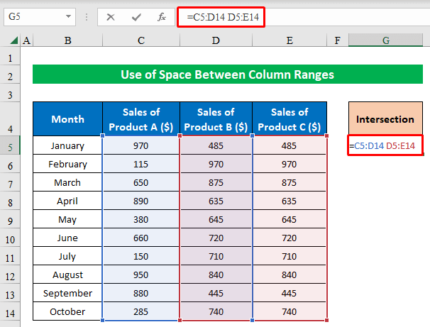
- Click ENTER to get the result.
- As you can see, we have extracted the intersection output in a new column.
Method 3 – Utilizing Named Ranges to Find the Intersection of Two Columns
Steps:
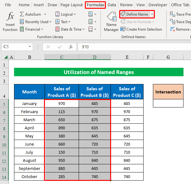
- Choose cells (C5:D14) and choose “Define Name” from the “Formulas” option.
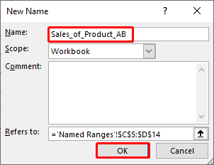
- Provide a name for the chosen column range in the “New Name” window and press OK.
- Select cells (D5:E14) and click “Define Name” from the “Formulas” tab.
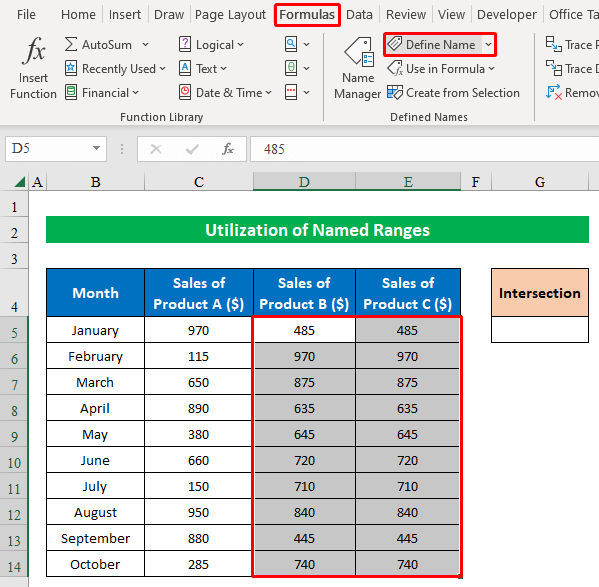
- Enter your desired name in the “Name” section and press OK.
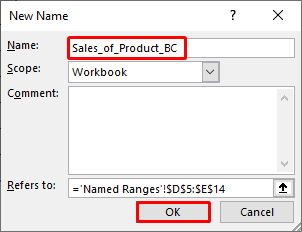
- Choose row-wise cells (B7:E7), provide a name in the “New Name” window, and click OK.
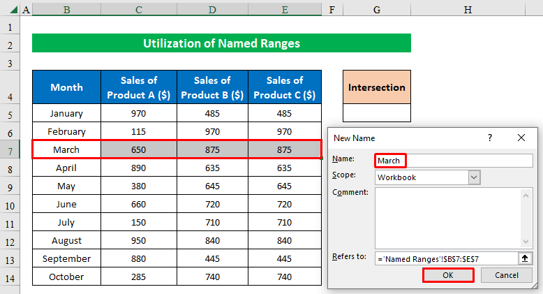
- After finishing naming columns and rows, apply the below formula in cell (G5) to find the intersection output:
=Sales_of_Product_AB:Sales_of_Product_BC March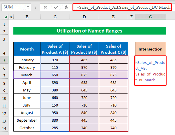
- Press ENTER.
- We have successfully extracted our intersection result from multiple columns within seconds.
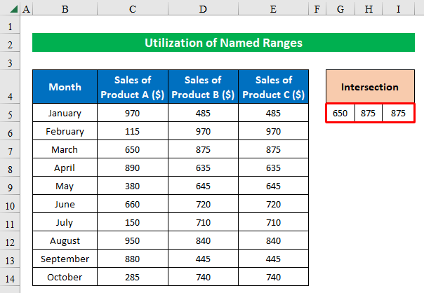
Read More: How to Use Intersection Operator in Excel
Method – Applying the VLOOKUP Function to Find Intersection Value
Steps:
- Choose a cell (G5) and enter the below formula:
=VLOOKUP(C5,$D$5:$D$14,1,0)Where,
- The VLOOKUP function will look for the given cell value in cell (C5) from a specific column range (D5:D14).
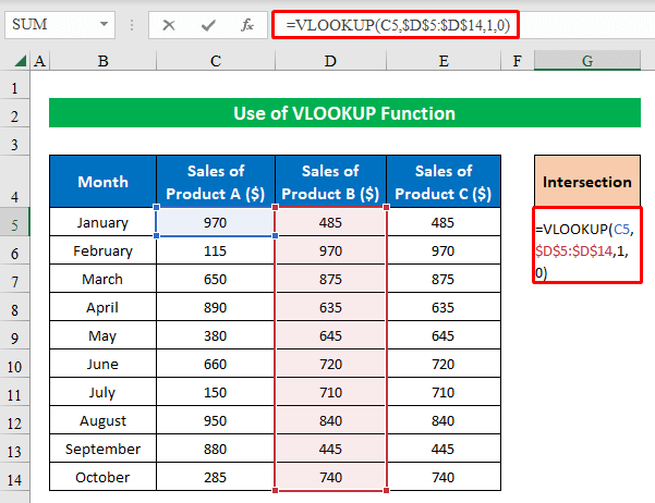
- Press ENTER.
- The VLOOKUP function will provide us with the intersection output in the chosen cell.
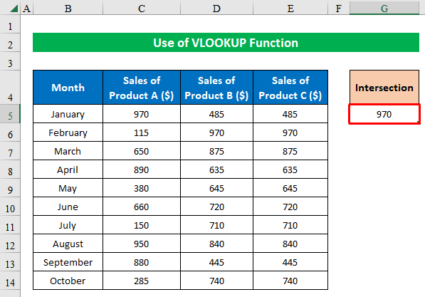
Method 5 – Using INDEX, SMALL, IF, COUNTIF, MATCH, ROW, and ROWS Functions
Steps:
- Select a cell (G5) and write the below formula:
=INDEX($C$5:$C$14, SMALL(IF(COUNTIF($D$5:$D$14, $C$5:$C$14), MATCH(ROW($C$5:$C$14),ROW($C$5:$C$14)), ""), ROWS($A$1:A1)))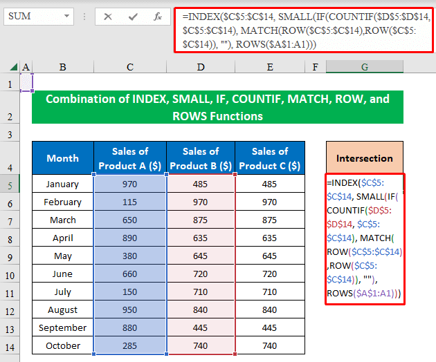
- Press ENTER to get the result.
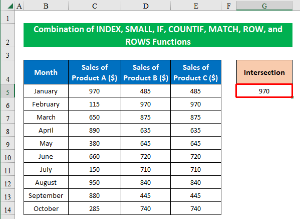
- You will get your desired result.
- The COUNTIF function will compare values within two columns (D5:D14) and (C5:C14) and return output as 1 or 0. The output stands as{1;0;0;0;0;0;0;0;0;0}.
- IF({1;0;0;0;0;0;0;0;0;0}, MATCH(ROW($C$5:$C$14),ROW($C$5:$C$14)), “”) → In this part, the ROW function will provide the cells row number inside the argument. Then the MATCH function will look for the position of the string. So, the result stands as- {1;””;””;””;””;””;””;””;””;””}
- SMALL(IF(COUNTIF($D$5:$D$14, $C$5:$C$14), MATCH(ROW($C$5:$C$14),ROW($C$5:$C$14)), “”), ROWS($A$1:A1)) → In this section, we extracted a specific number from an array using the SMALL function returning 1.
- INDEX($C$5:$C$14, SMALL(IF(COUNTIF($D$5:$D$14, $C$5:$C$14), MATCH(ROW($C$5:$C$14),ROW($C$5:$C$14)), “”), ROWS($A$1:A1))) → In this final part, the INDEX function will provide the cell value from a particular location in cell range (C5:C14). Thus the final result stands as 970.
Method 6 – Combining FILTER and COUNTIF Functions
Steps:
- Choose a cell (G5) and apply the below formula:
=FILTER($C$5:$C$14,COUNTIF($D$5:$D$14, $C$5:$C$14))Where,
- The COUNTIF function will provide compared values from the given column ranges in the string.
- The FILTER function will return cell values from the given condition.
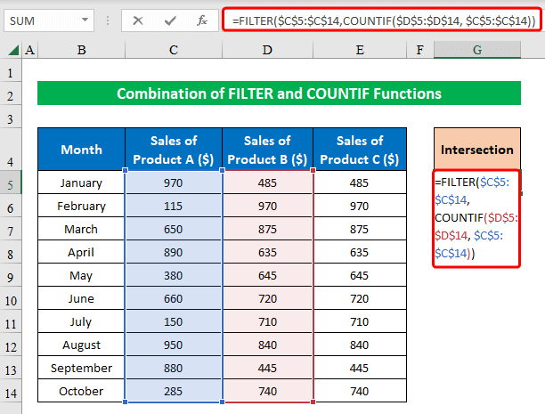
- Click ENTER and get your precious intersected values in a new column.

Method 7 – Using FILTER, MMULT, EXACT, TRANSPOSE, and ROW Functions
Steps:
- Choose a cell (G5) and apply the below formula:
=FILTER($C$5:$C$14,MMULT(EXACT(C5:C14,TRANSPOSE(D5:D14))*1,ROW(C5:C14)^0))Where,
- The ROW function will return the row number as {5;6;7;8;9;10;11;12;13;14} from the specified cell range C5:C14.
- The TRANSPOSE function will convert the vertical range of cells to a horizontal array.
- The EXACT function will perform a case-sensitive comparison between values.
- The MMULT function returns the matrix product of two arrays, and finally, the FILTER function provides the cell value from the given matrix condition.
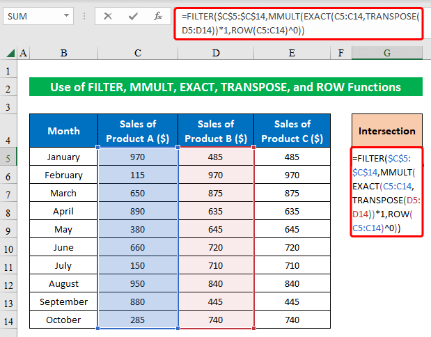
- Click ENTER.
- You will get the intersection output of two columns in Excel.

Download the Practice Workbook
Download this workbook to practice.
<< Go Back to Excel Operators | Excel Formulas | Learn Excel
Get FREE Advanced Excel Exercises with Solutions!

