There are 2 worksheets: Sheet1 and Sheet2.
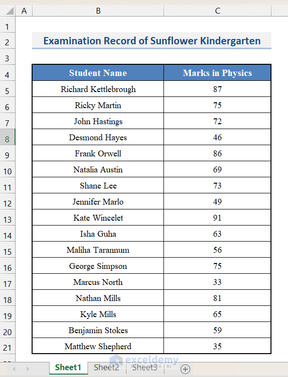
In Sheet1, you have students’ marks in Physics.
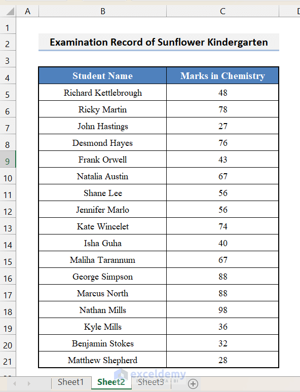
In Sheet2, students’ marks in Chemistry .
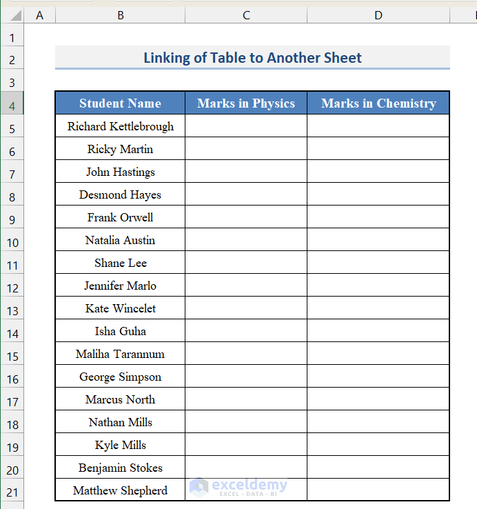
Create a table in another worksheet to link the marks in Physics and Chemistry:
Method 1 – Using the Worksheet Names in the Formula to Link the Tables
Steps:
- Go to the worksheet containing the data table.
- Select the top cell in a column. Here, C5 (the first cell in the Physics column).
- To link C5 from Sheet1, enter an equal sign (=) in the cell in a new sheet.
- Go back to Sheet1, select C5 and press Enter.
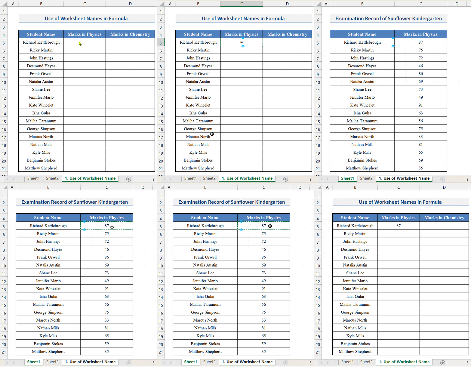
- You will see the value of C5 from Sheet1 in this cell.
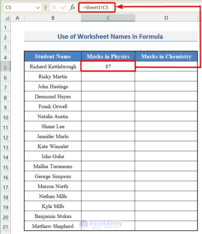
- C5 in this table is linked to C5 in Sheet1. If you make any changes in C5 in Sheet1, the changes will reflect on this cell.
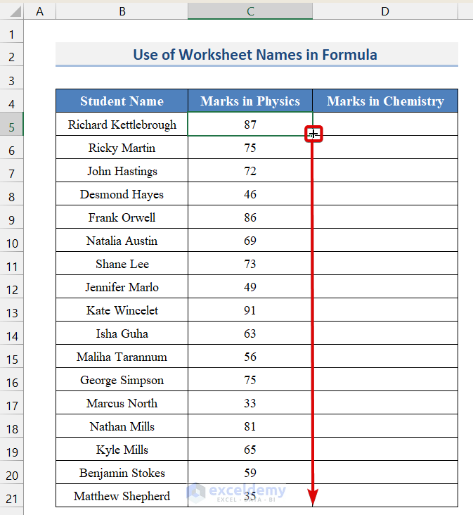
- Drag down the Fill Handle to autofill the rest of the cells in the Physics column.
- Follow the same steps for the marks in Chemistry.
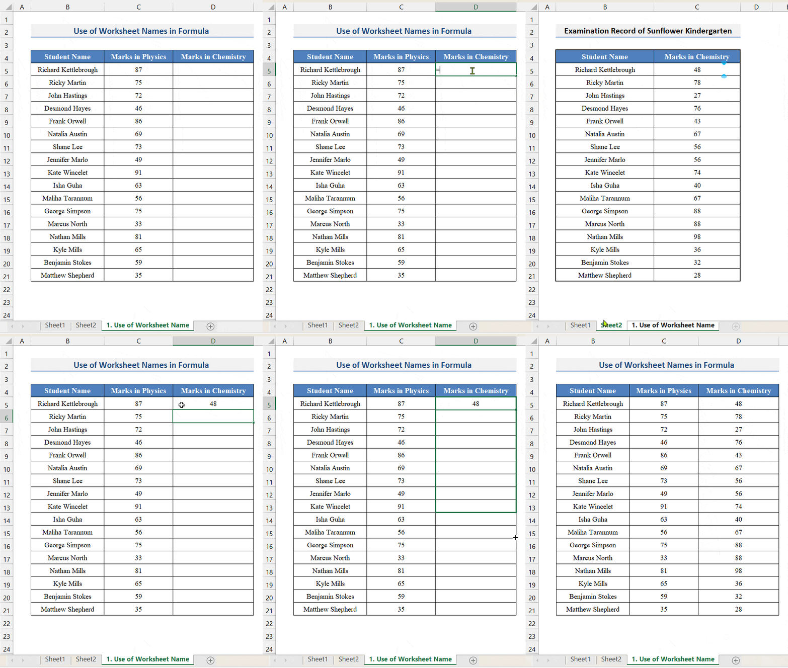
- You can also manually enter the Sheet name in the formula. The syntax will be:
If you have a space or punctuation marks in your referred worksheet name, you must enclose the worksheet name within a single quotation.
To use a table:
- Select the dataset and click Ctrl+L.
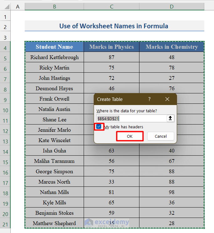
- Check My table has headers and click OK.
The whole dataset will be converted into an Excel Table. The table contains the linked cells of the other sheets.
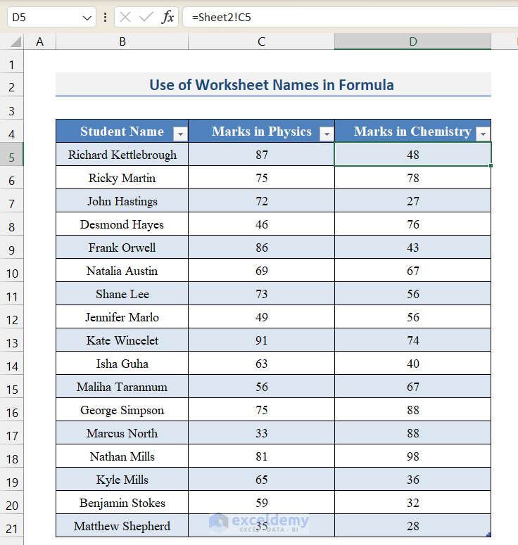
Method 2 – Linking a Table by Creating a Hyperlink
2.1 Using the HYPERLINK Function to create a Hyperlink
Steps:
- To create a hyperlink with the marks of Physics in Sheet2, enter this formula in C5 and press Enter.
=HYPERLINK("#Sheet1!C5","Marks")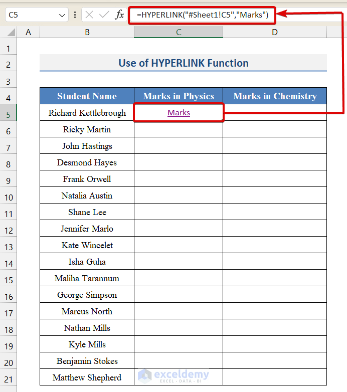
-
- “#Sheet1!C5” indicates you want to link to C5 of Sheet1
- The Hash (#) symbol indicates the worksheet is in the same workbook.
- “Marks” is the name of the link that will be displayed.
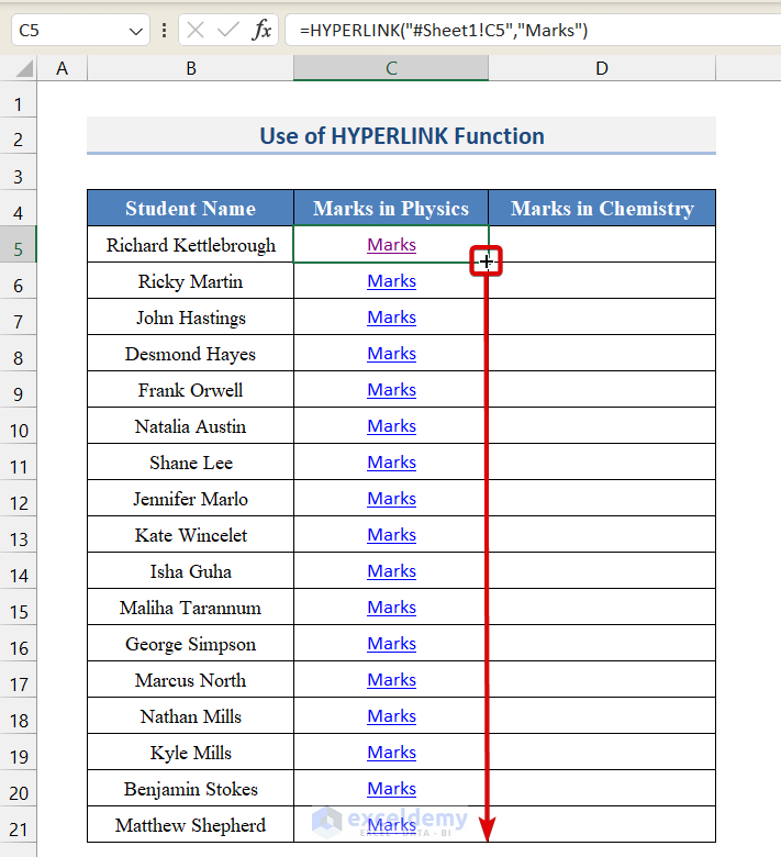
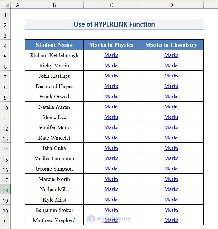
- Drag down the Fill Handle to create a link for all students.
- If you click the linked cells, the link will lead you to Sheet1.
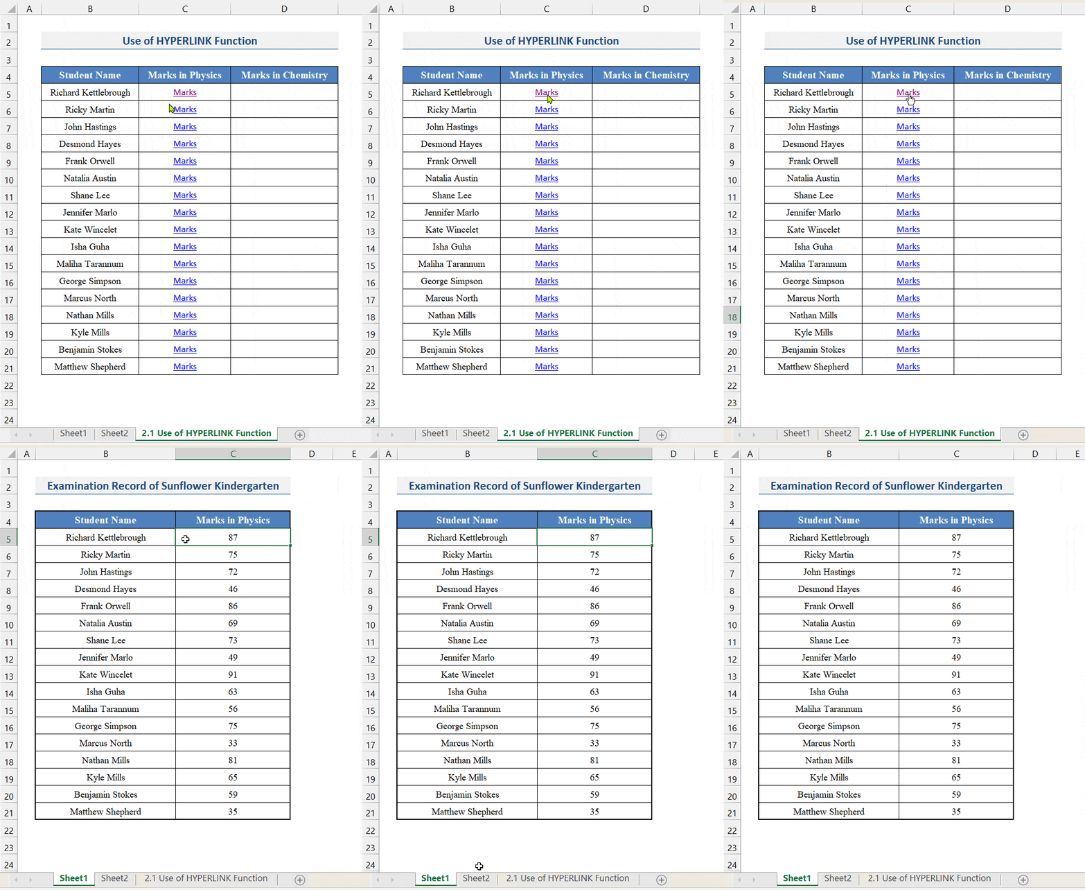
- Repeat the procedure for the marks in Chemistry Sheet2. The formula in the first cell in the Chemistry column is:
=HYPERLINK("#Sheet2!C5","Marks")This is the output.
Read More: How to Link Sheets in Excel with a Formula
2.2 Create a Hyperlink using the Context Menu
Steps:
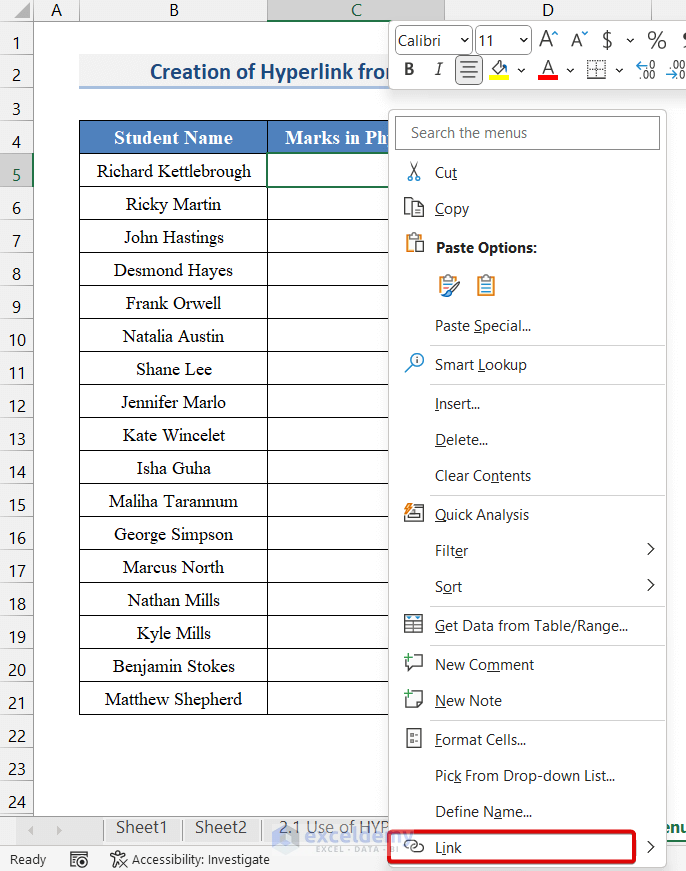
- Select the cell to enter the hyperlink.
- Right-click and choose Link.
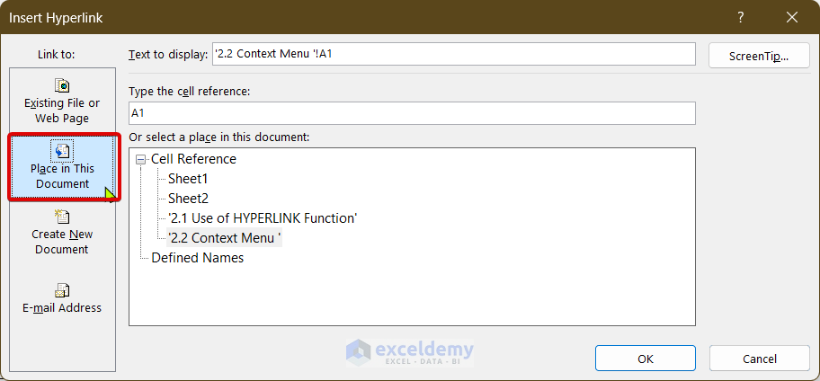
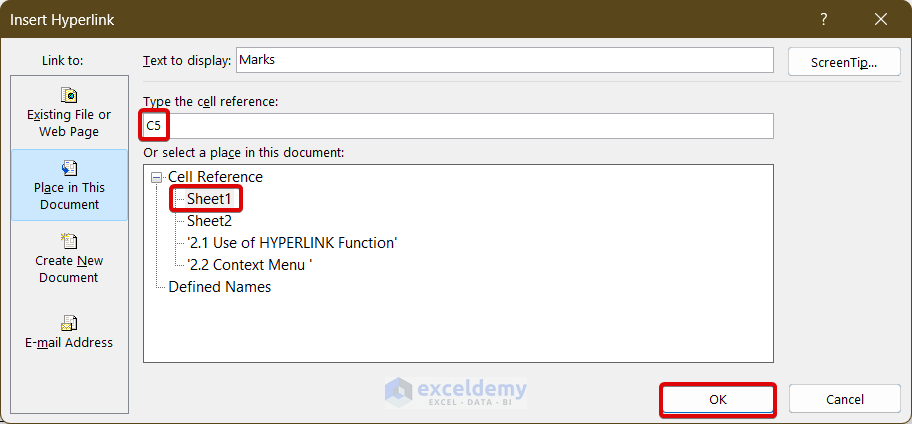
- In the Insert Hyperlink dialog box, select Place in this Document.
- In Text to Display, enter the name of the link. Here, Marks.
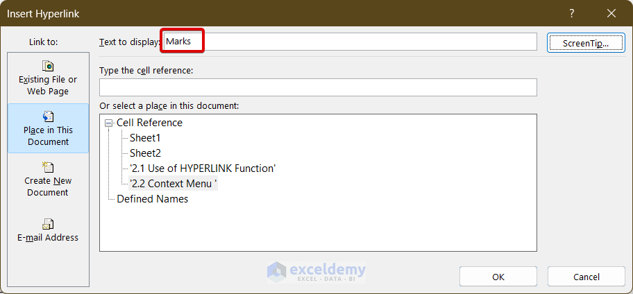
- In Type the Cell Reference box, enter the cell reference. Here, C5.
- In Select a Place in the Document, select the worksheet name to which you want to link. Here, Sheet1.
The “Marks” hyperlink is created.
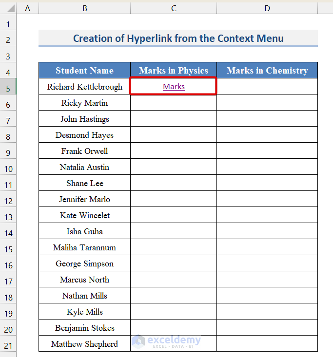
If you click it, you will be directed to the linked cell (C5 in Sheet1).
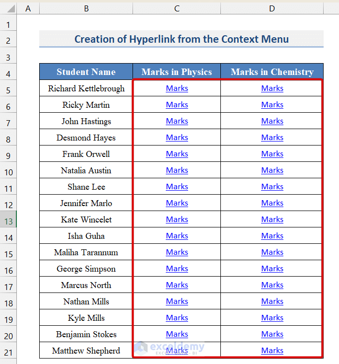
- Repeat the procedure for the rest of the cells.
Read More: How to Link Sheets to a Master Sheet in Excel
Download Practice Workbook
Download the practice workbook.
Related Articles
- How to Link Cell to Another Sheet in Excel
- How to Link Two Sheets in Excel
- How to Link Excel Data Across Multiple Sheets
- How to Link Data in Excel from One Sheet to Another
<< Go Back To Excel Link Sheets | Linking in Excel | Learn Excel
Get FREE Advanced Excel Exercises with Solutions!

