Serial numbers are important for sorting, ordering, and maintaining the consistency of data in Excel. In this article, you will learn how to create a serial number in Excel using built-in features and formulas.
Method 1 – Add Serial Number in Excel with Built-in Features
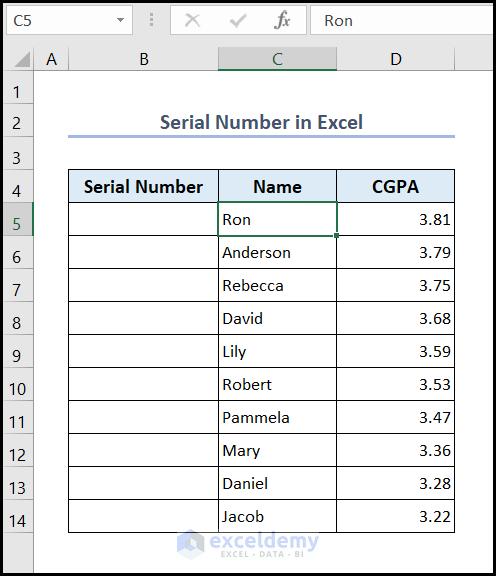
The dataset below has the Names and CGPAs of multiple students, but the Serial Number column is blank. We will generate serial numbers using the built-in features of Excel.
Example 1 – Use the Fill Handle Feature
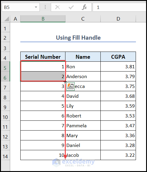
- Enter 1 in cell B5 and 2 in cell B6.
- Select range B5:B6 and use Fill Handle to AutoFill data in range B7:B14.
Example 2 – Apply the Fill Series Option of Excel
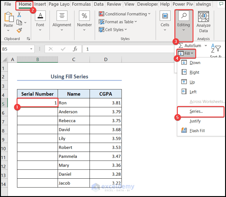
- Enter 1 in cell B5.
- Go to the Home tab and select the Fill option from the Editing group.
- Select Series from the drop-down menu of Fill.
- From the Series dialog box, select the Columns series and put 10 as the Stop value. Click OK.
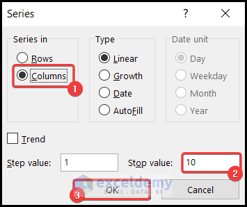
Note: The Step value is set to 1 by default.
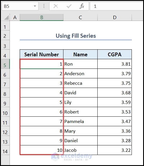
- It will output serial numbers in the dataset.
Method 2 – Use Formula to Add Serial Number in Excel
Example 1 – Use Excel SEQUENCE Function
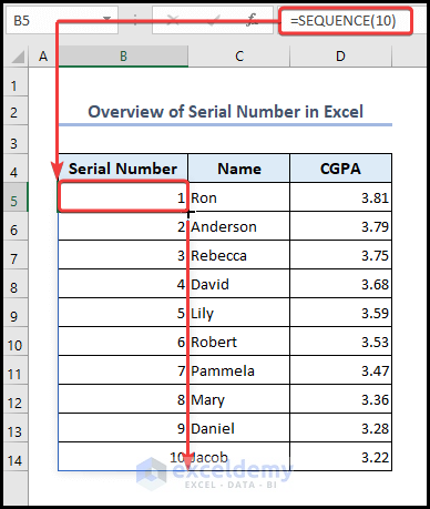
- Select cell B5 and enter the formula based on the SEQUENCE function into this cell.
- Press Enter.
=SEQUENCE(10)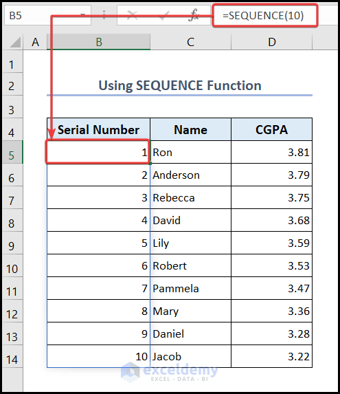
Example 2 – Use the ROW Function to Serial Number in Excel
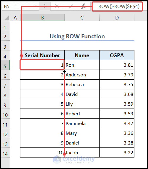
- Go to cell B5 and insert the following formula based on the ROW function.
=ROW()-ROW($B$4)- Press Enter and use the Fill Handle to AutoFill data in range B6:B14.
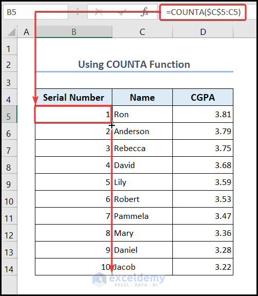
Example 3 – Apply the COUNTA Function for Serial Numbers
- Go to cell B5 and insert the below formula based on the COUNTA function.
=COUNTA($C$5:C5)- Press Enter and use the Fill Handle to AutoFill data in range B6:B14.
Read More: Automatically Number Columns in Excel
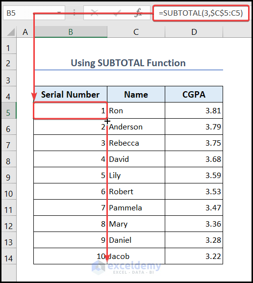
Example 4 – Use the SUBTOTAL Function for Serial Numbers
- Go to cell B5 and insert the following formula based on the SUBTOTAL function.
=SUBTOTAL(3,$C$5:C5)- Press Enter and use the Fill Handle to AutoFill data in range B6:B14.
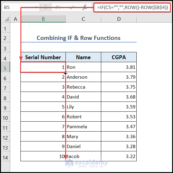
Example 5 – Combine IF and ROW Functions
- Go to cell B5 and insert a formula based on the combination of IF and ROW functions.
=IF(C5="","",ROW()-ROW($B$4))- Press Enter and use the Fill Handle to AutoFill data in range B6:B14.
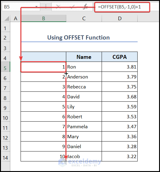
Example 6 – Use of OFFSET Function to Add Serial Number in Excel
- Go to cell B5 and insert the following formula based on the OFFSET function.
=OFFSET(B5,-1,0)+1- Press Enter and use the Fill Handle to AutoFill data in range B6:B14.
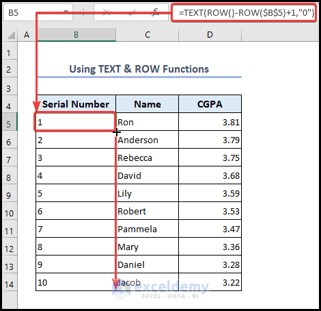
Example 7 – Combination of ROW and TEXT Functions for Serial Numbers
- Go to cell B5 and insert a formula based on the combination of ROW and TEXT functions.
=TEXT(ROW()-ROW($B$5)+1,"0")- Press Enter and use the Fill Handle to AutoFill data in range B6:B14.
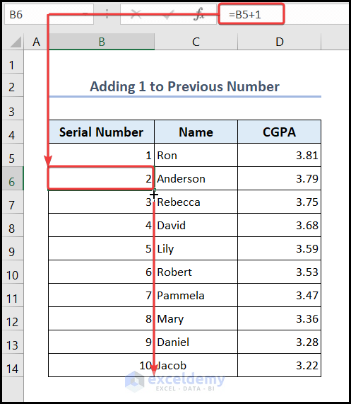
Example 8 – Add 1 to the Previous Number to Get the Serial Number of Cells
- Enter 1 in cell B5.
- Go to cell B6 and put this formula into the cell.
=B5+1- Press Enter and use the Fill Handle to AutoFill data in range B7:B14.
Read More: Auto Generate Serial Number Using Excel VBA
Method 3 – Insert Serial Number Using Other Features of Excel
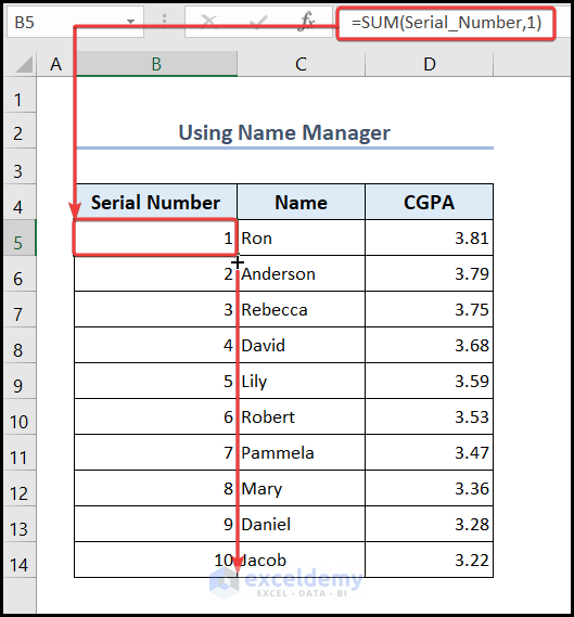
Example 1 – Use Excel Name Manager to Get Serial Numbers
- Go to Formulas tab >> Define Name.

- In the New Name dialog box, add a name. We have added Serial_Number.
- Enter the following formula in the Refers to box and press OK.
=INDIRECT("R[-1]C",FALSE)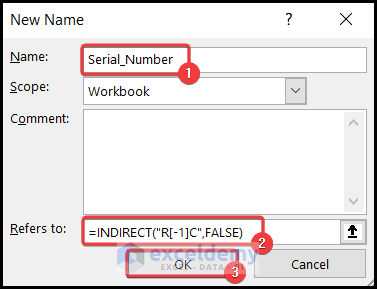
- Go to cell B5 and insert the formula based on the SUM function.
=SUM(Serial_Number,1)- Press Enter and use the Fill Handle to AutoFill data in range B6:B14.
Example 2 – Insert Dynamic Serial Numbers for Filters
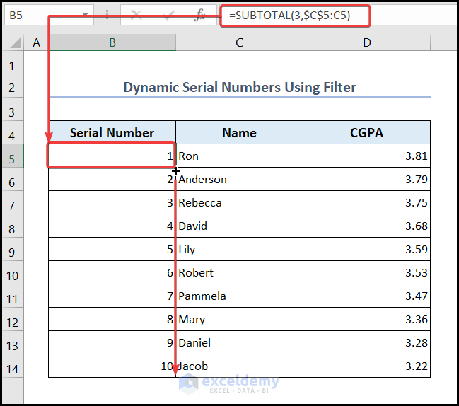
- Go to cell B5 and insert the following formula.
=SUBTOTAL(3,$C$5:C5)- Press Enter and use the Fill Handle to AutoFill data in range B6:B14.
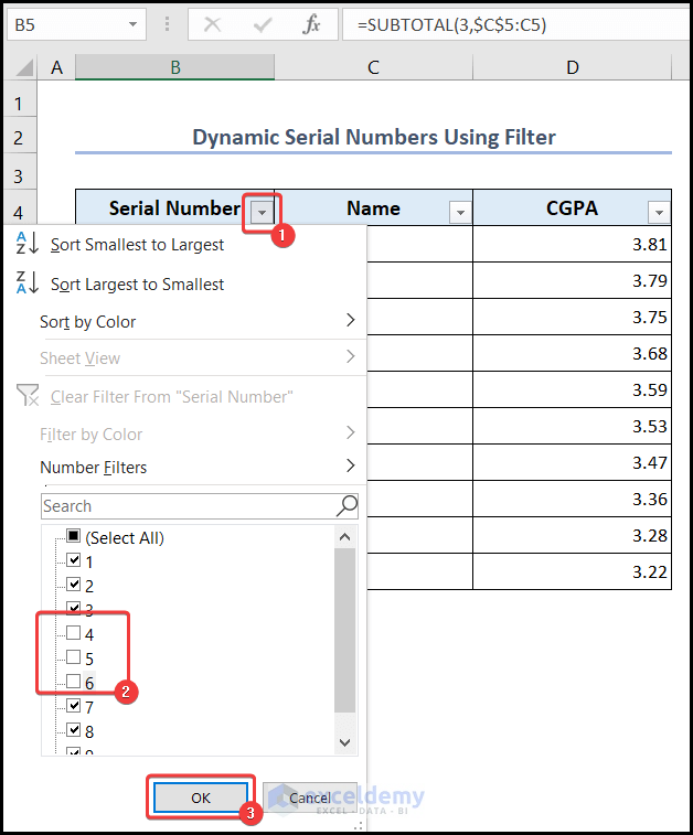
- Select Sort & Filter from the Home tab. Click on the Filter option from the drop-down menu.

- Click on a drop-down arrow and apply the filter according to your preference. We have unchecked serial numbers 4, 5, 6.
- Press OK to proceed.
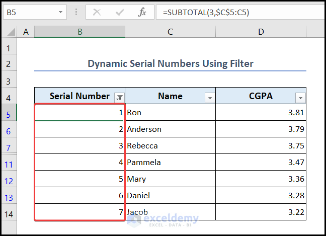
- The serial numbers will be updated.
Read More: Automatically Number Rows in Excel
Example 3 – Automatically Add Serial Number in an Excel Table
- Enter 1 in cell B5.
- Go to cell B6 and insert this formula.
=B5+1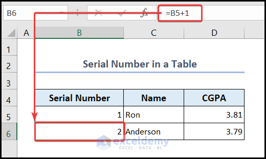
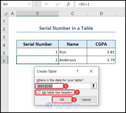
- Press Ctrl+T to open the Create Table dialog box.
- Put range $B$4:$D$6 in the box of the Create Table dialog box. Check the My table has headers option and press OK.
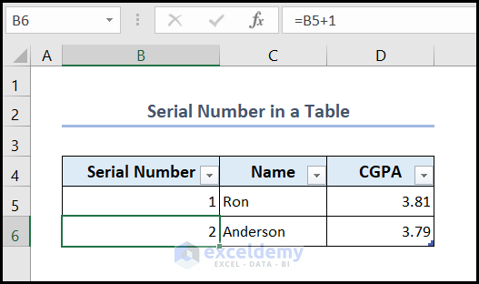
- A table will be created with the dataset.
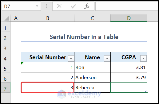
- Enter Rebecca in cell C7 and press the Tab
- You will see the serial number is generated automatically.
Example 4 – Serial Number in a Pivot Table
- Add a new column in the source data with 1 in each cell.
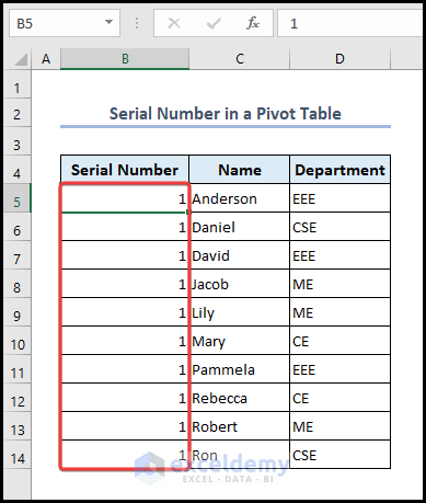
- Select a cell in the table.
- Go to Insert tab >> Pivot Table >> From Table/Range option.
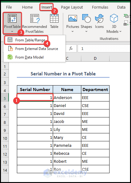
- You will see the source data range is added automatically in the Table/Range section.
- Set the location of the pivot table in the dialog box and press OK.
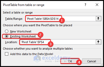
- A pivot table will be created.
- Check and place the Serial Number and Name in the PivotTable Fields as shown in the image below.
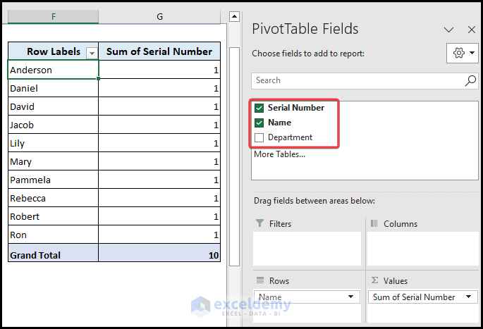
- Click on Sum of Serial Numbers below and select Value Field Settings.
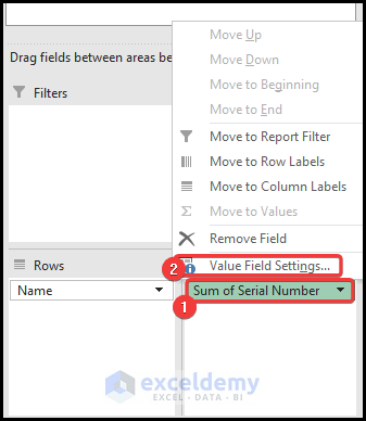
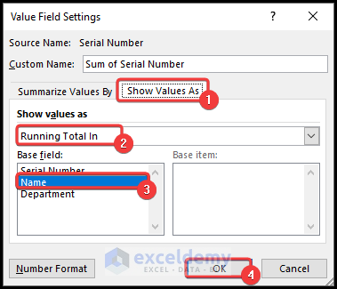
- Set up the dialog box as shown: Value Field Settings dialog box >> open the Show Values As tab >> select the Running Total In option from the drop-down list >> select Name as the Base field >> click OK.
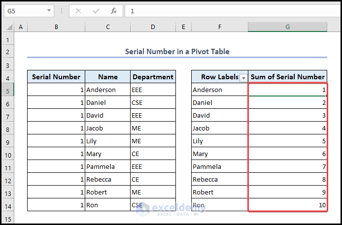
- You will see a pivot table with serial numbers.
Example 5 – Use Power Pivot to Add Serial Number
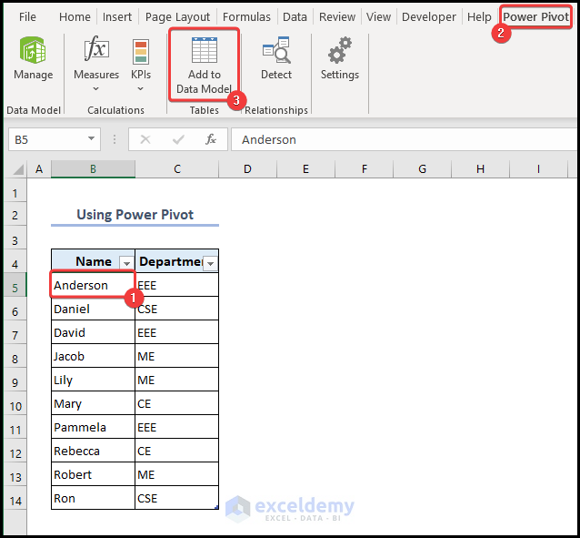
- Select a cell in your dataset.
- Go to Power Pivot >> Add to Data Model.
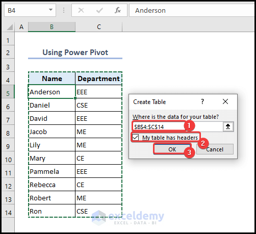
- Check the range shown in the Create Table window.
- Check My table has headers option and press OK.
- This will open a power query window.
- Add a column named Index and put the formula in the first cell of the column.
=RANK.EQ( Table8[Name], Table8[Name], ASC )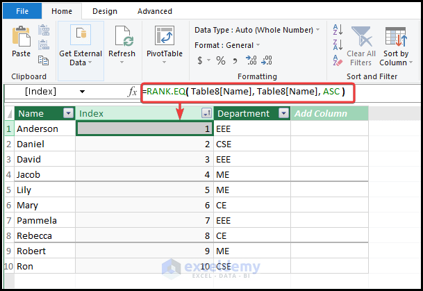
Table8 is the name of the data model table and we are ranking based on the name.
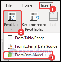
- Go to Insert tab >> Pivot Table >> From Data Model option.
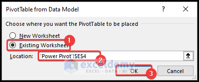
- Select the location of the pivot table and press OK.
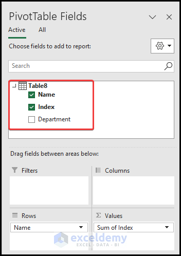
- In the PivotTable Fields, select Name and Index from Table8.
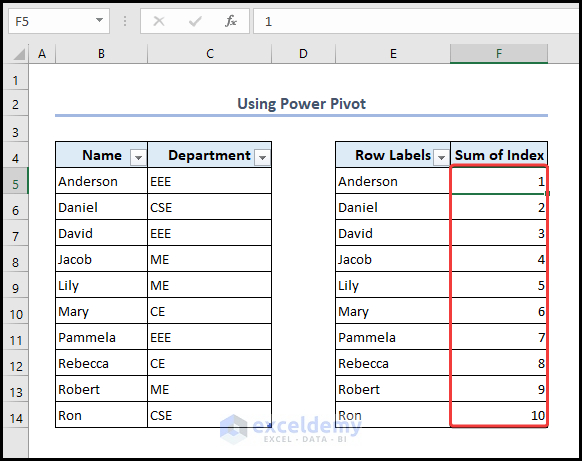
- You will see the pivot table with the serial number in the Sum of Index column.
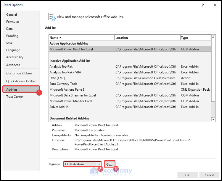
Note: Power Pivot is not available in all versions of Excel. It is available from Excel 2013 to the latest versions. To find it in your version follow these steps:
- Go to File >> Options >> Add-ins.
- Select COM Add-ins and press Go.
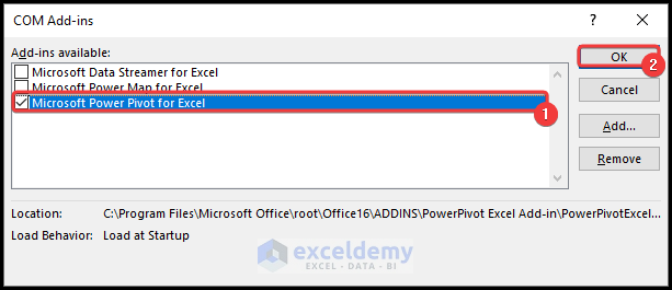
- If you have the Power Pivot in your version of Excel, you will see Microsoft Power Pivot for Excel in your dialog box. Check it and press OK.
Example 6 – Add Serial Numbers Using Index Column in Power Query
- Select a cell of your table.
- Go to the Data tab >> From Table/Range.
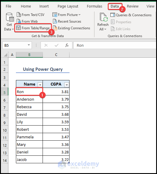
- This will open up the Power Query Editor.
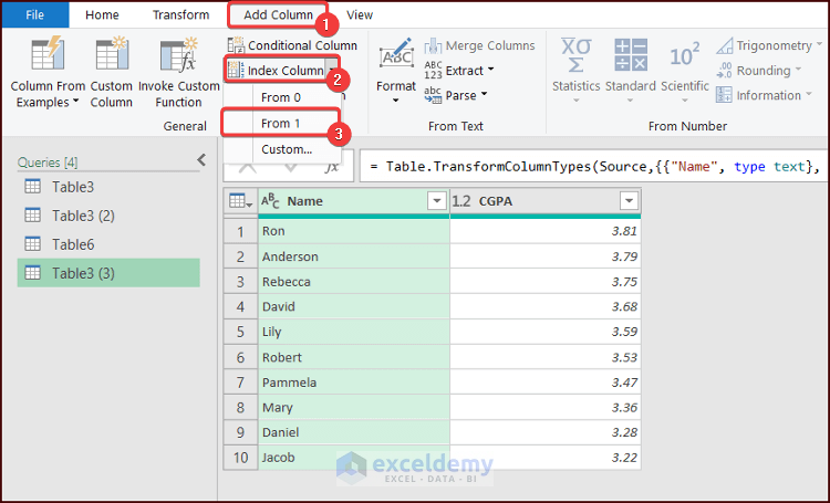
- Go to Add Column tab >> Index Column command >> From 1.
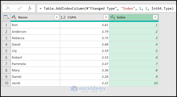
- You will see the dataset with the Index column.
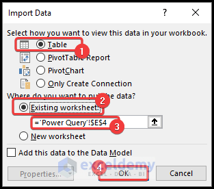
- Go to Home tab >> Close & Load >> Close and Load to.

- Select the location of the table and press OK.
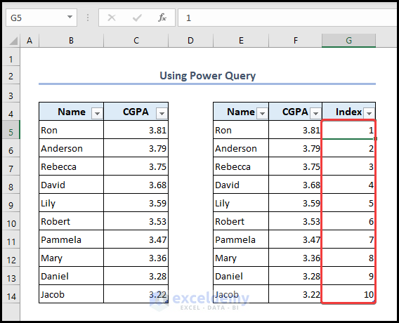
- You will see an additional table with an Index column.
Example 7 – Use the Connection Properties for Connected Tables
- Create a connected table.
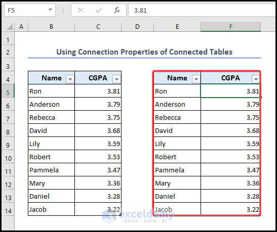
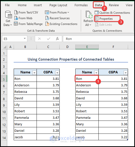
- Select any cell of your connected table.
- Go to the Data tab >> Properties.
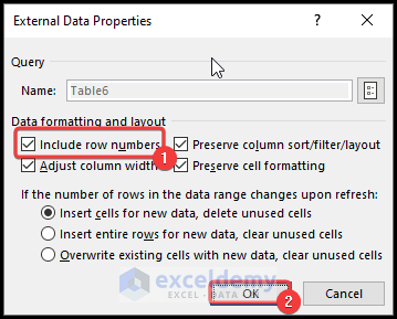
- Check the Include row numbers option and press OK.
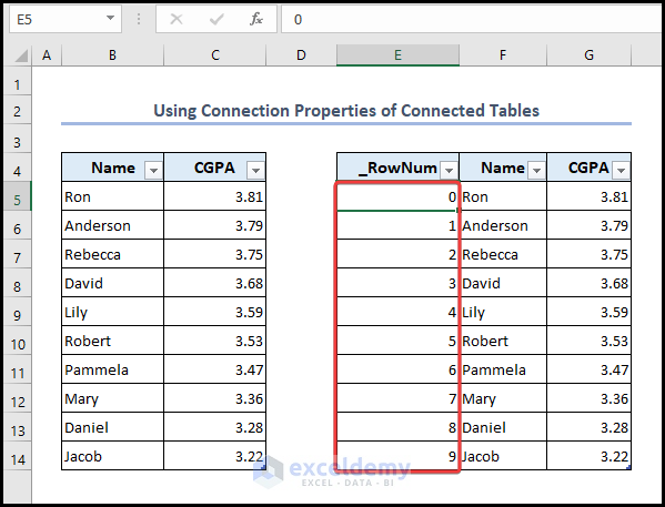
- Go to the Data tab >> press Refresh.

- You will see the serial number starting from 0.
Method 4 – Add Serial Number with VBA Code
- Go to the Developer tab >> Visual Basic.

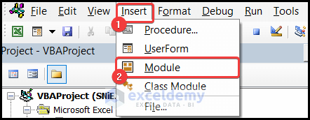
- Go to Insert >> Module.
- Put the following code in your VBA Macro Editor and press the Run key or F5 to run the code.
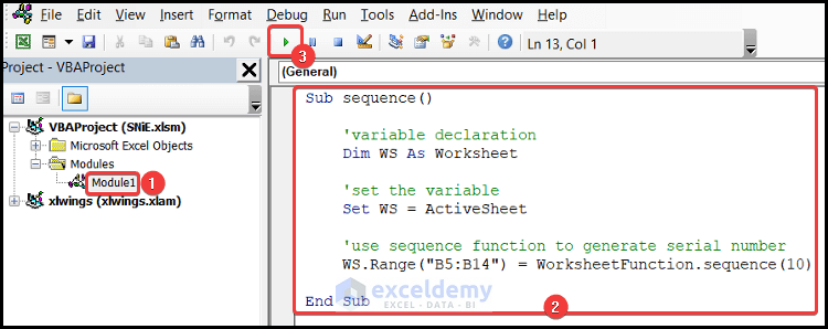
Sub sequence()
    'variable declaration
    Dim WS As Worksheet
    'set the variable
    Set WS = ActiveSheet
    'use sequence function to generate serial number
    WS.Range("B5:B14") = WorksheetFunction.sequence(10)
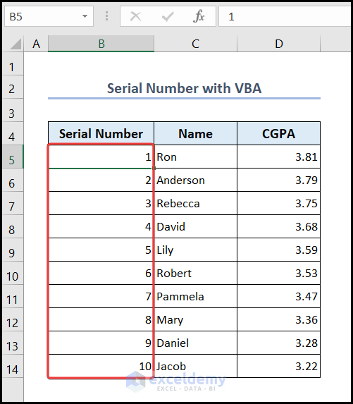
End Sub- You will see the serial number in your dataset.
Read More: Auto Serial Number Based on Another Column
Method 5 – Examples of Inserting Serial Numbers in Practical Life
Example 1 – Add Roman Numbers as Serial Numbers
- Go to cell B5 and insert a formula based on the combination of ROMAN and ROW
=ROMAN(ROW()-ROW($B$4))- Press Enter and use the Fill Handle to AutoFill data in range B6:B14.
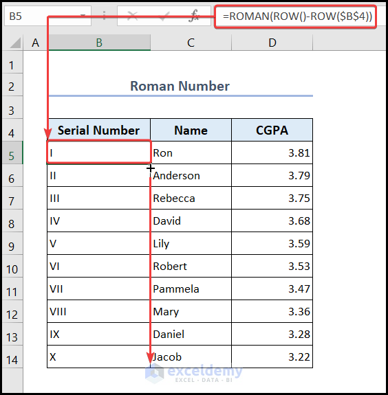
Note: The ROMAN function converts the numeric number you get from the ROW function.
2. Add a Serial Dates in a Column
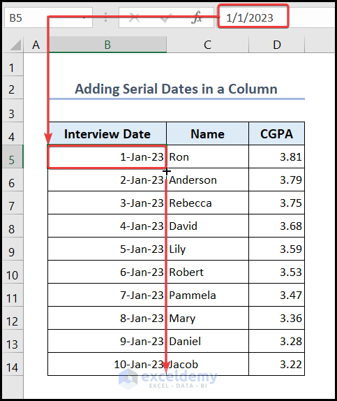
In the dataset, we have the Names and CGPAs of students. Data are sorted in descending order of CGPA. The interview date will be in a serial according to their CGPAs.
- Go to cell B5 and insert the date.
=1/1/2023- Press Enter and use the Fill Handle to AutoFill data in range B6:B14.
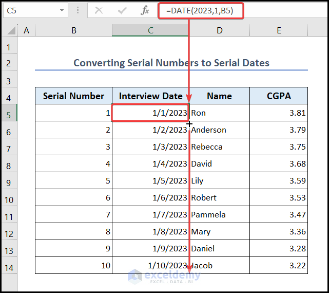
Example 3 – Convert Serial Numbers to Serial Dates
- Go to cell C5 and insert the formula based on the DATE function.
=DATE(2023,1,B5)- Press Enter and use the Fill Handle to AutoFill data in range C6:C14.
Things to Remember
- You may need to put the initial value.
- While using Fill Handle, be aware that the step number is always 1. If you want a custom step number, you can use the Fill Series option.
- While using the OFFSET function, make sure that the cell above the one where you put the formula is blank.
Download Practice Workbook
Frequently Asked Questions
1. Can I generate alphanumeric serial numbers in Excel?
Yes, you can generate alphanumeric serial numbers in Excel. You can combine the ROW function with other functions like the CHAR function to convert numbers to corresponding characters.
2. Is it possible to automatically increment the serial number when adding new rows or entries?
Yes, it is possible to automatically increment the serial number when adding new rows or entries. You can use formulas that dynamically update based on the number of rows or entries in your data range. You can also use Excel Table.
3. Is there a way to generate random serial numbers in Excel?
Yes, you can generate random serial numbers in Excel using the RAND function or by creating a custom VBA macro that generates random numbers within a specific range.
Serial Number in Excel: Knowledge Hub
<< Go Back to Numbering in Excel | Learn Excel
Get FREE Advanced Excel Exercises with Solutions!

