Method 1 – Combine Rows with the Same ID using VBA
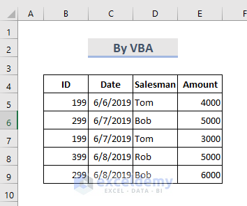
This is the sample dataset.
To merge values:
STEPS:
- Go to the Sheet tab and right-click.
- Select View Code.
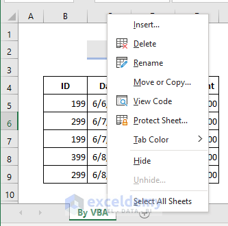
- The Microsoft Visual Basic for Application window is displayed.
Note: You can also find this window also by pressing Alt+F11.
- In the module window, use the following VBA code.
Sub Combine_Rows_with_IDs()
Dim x1 As Range
Dim x2 As Long
Dim A As Long, B As Long, C As Long
On Error Resume Next
Set x1 = Application.InputBox("Select Range:", "Combine Rows with IDs", Selection.Address, , , , , 8)
Set x1 = Range(Intersect(x1, ActiveSheet.UsedRange).Address)
If x1 Is Nothing Then Exit Sub
x2 = x1.Rows.Count
For A = x2 To 2 Step -1
For B = 1 To A - 1
If x1(A, 1).Value = x1(B, 1).Value And B <> A Then
For C = 2 To x1.Columns.Count
If x1(B, C).Value <> "" Then
If x1(A, C).Value = "" Then
x1(A, C) = x1(B, C).Value
Else
x1(A, C) = x1(A, C).Value & "," & x1(B, C).Value
End If
End If
Next
x1(B, 1).EntireRow.Delete
A = A - 1
B = B - 1
End If
Next
Next
ActiveSheet.UsedRange.Columns.AutoFit
End Sub- Click Run button or press F5.
- In the dialog box, select the rows you want to combine.
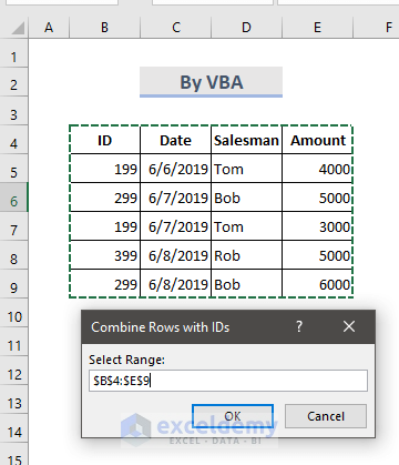
- Click OK.
- This is the output.
Method 2 – Using the Consolidate Tool to Merge Rows in Excel
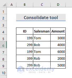
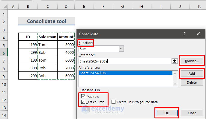
The worksheet contains name and salary. To find the total amount of a salesman’s salary:
STEPS:
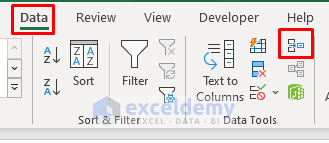
- In the Toolbar, select Data > Consolidate.
- In the dialog box, choose a Function.
- Select the data range.
- Click Add to add the references.
- Check Top row and Left column and click OK.
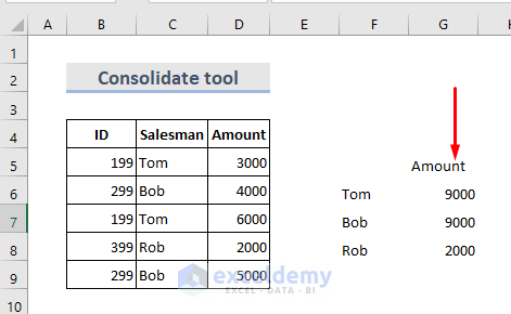
- This is the output.
Method 3 – Using the IF Function to Combine Rows in Excel
The dataset contains books in different rows.

STEPS:
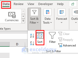
- Select the table, click Data > Sort.
- Sort the table by the main column.
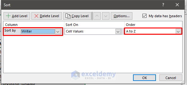
- This is the output.

- Create helping columns to containing the formula to merge the book name.
- In D5, enter the formula:
=IF(B5=B4,D4&", "&C5,C5)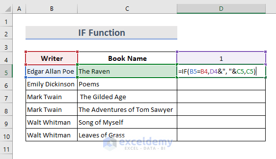
- Press Enter.
- Drag down the Fill Handle to see the result in the rest of the cells.

- Create another column and use another formula to complete the book name listing.
- In E5, enter the formula:
=IF(B6<>B5,"Merged","")
- Press Enter.
- Drag down the Fill Handle to see the result in the rest of the cells.

- Copy the results and paste them into D5 as values.
- Sort the values by the last helping column in descending order.
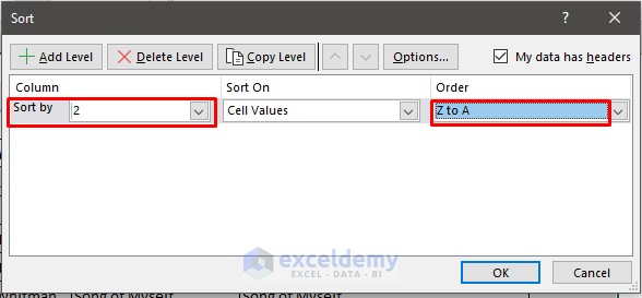
- This is the output.

- Delete the helping column.
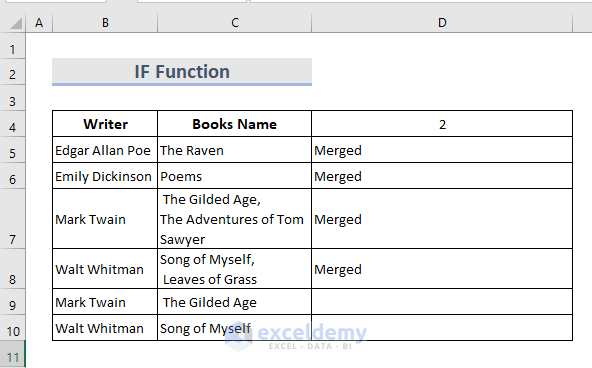
Practice Workbook
Download the following workbook and exercise.
Related Readings
- How to Combine Multiple Rows into One Cell in Excel
- How to Merge Rows Based on Criteria in Excel
- How to Merge Rows with Same Value in Excel
- How to Merge Rows and Columns in Excel
- How to Convert Multiple Rows to a Single Column in Excel
- How to Convert Multiple Rows to Single Row in Excel
- How to Merge Rows Without Losing Data in Excel
- How to Merge Two Rows in Excel
- How to Merge Rows with Comma in Excel
<< Go Back to Merge Rows in Excel | Merge in Excel | Learn Excel
Get FREE Advanced Excel Exercises with Solutions!


This helped me a great deal. It was very difficult to find a clean solution for this problem and I ended up using the #3. Thanks very much.
It’s great to hear you liked the article. You are most welcome. Best wishes.