How to Sum in Excel (All Things You Need to Know)

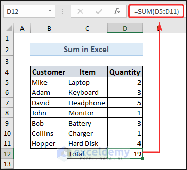
Here’s the simplest use of the SUM function to sum a range of values.

Download the Practice Workbook

Example 1 – Sum a Range of Cells with AutoSum Feature

• Select a cell where you want to apply AutoSum.
• Go to the Home tab.
• Click AutoSum under the Editing group.

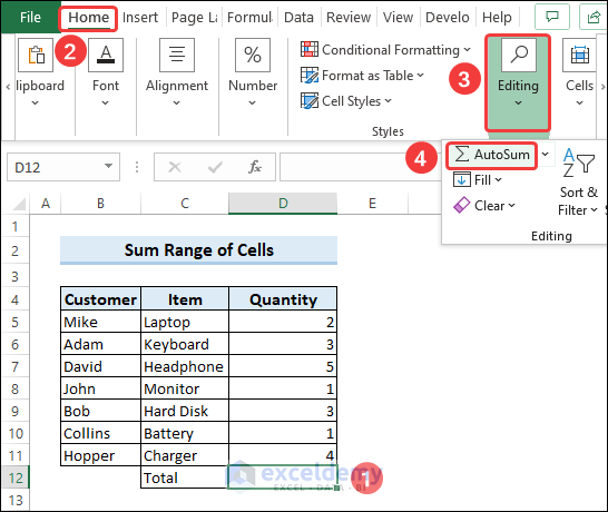
• This will insert the SUM formula.
• Press Enter.

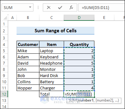
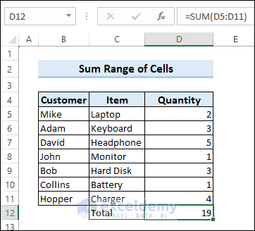
Excel will automatically calculate the sum of the range.

Example 2 – Sum Selected Cells from Excel Properties

• Click on the column name that contains your data.
• At the bottom section of the worksheet window, Excel will show you some properties of the selected range. You can get the sum from here.

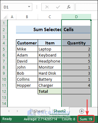
Example 3 – Sum a Range or Entire Column in Excel

• Apply the following formula to calculate the sum of the range D5 to D11.

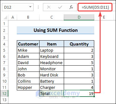
Example 4 – Find a Sum of Filtered Cells with the SUBTOTAL Function

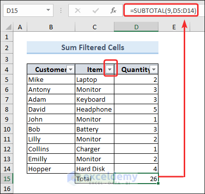
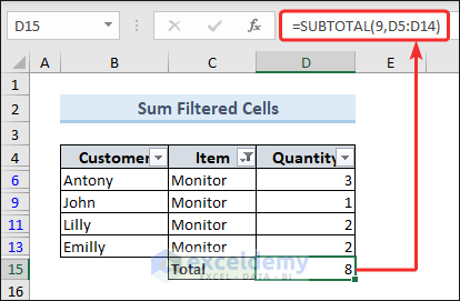
• For a filtered range of cells, we have applied the SUBTOTAL function to find the sum.

We found the Total Quantity => 26.

We want to find the sum of Monitor only, so we need to filter the Item column for Monitor.

• Click on the filter icon (the dropdown arrow) on the Item column.

• Mark only Monitor and click OK.

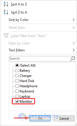
• This command will calculate the sum only for Monitor. So the total output will be decreased as now the concerning item is only the Monitor.

Example 5 – Convert a Range to a Table for Calculating a Sum

• Select a random cell in the range.
• Go to the Insert tab and click Table.

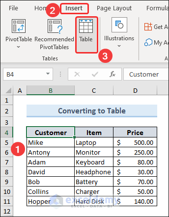
• Click OK on the Create Table dialog box.

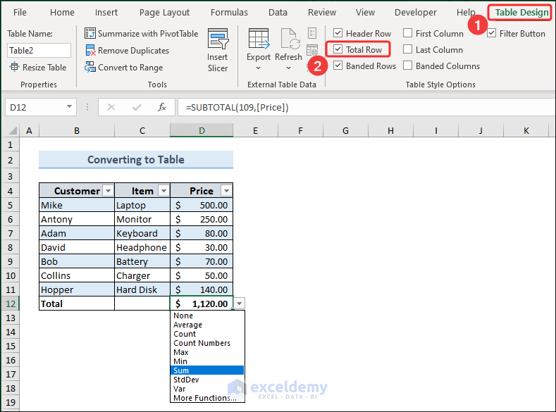
• After creating a Table, go to the Table Design tab and put a checkmark on Total Row.

This will insert a new column that will show you the sum of the numbers.

Example 6 – Calculate the Sum of Running Factors

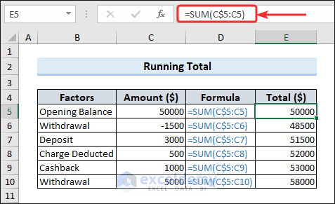
The dataset below represents the statement of a balance sheet. In column B, we have some transactions.

• Use the formula below for the first factor.

• Drag the Fill Handle tool down. This will Autofill the formula and calculate the running total for the factors.

Example 7 – Calculate a Sum Based on a Condition in Excel

Case 1 – Use the SUMIF Function to Match Single Criterion

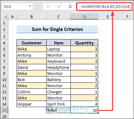
We want to get the sum of product quantity for Mike. So, we have only a single criterion here.

• The SUMIF function calculates the sum for a range based on a single criterion.

This formula calculates the sum in the range D5:D14 based on the cell value of B5.

Case 2 – Use the SUMIFS Function to Match Multiple Criteria

• If you want to calculate the total quantity of Monitor purchased by Mike, in that case, you can use the SUMIFS function.

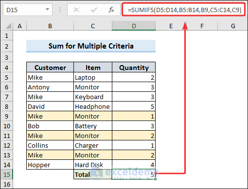
Example 8 – Sum Every N-th Row in Excel

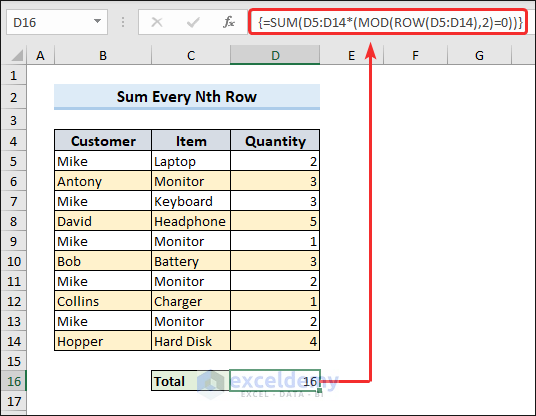
• Apply the following formula to sum every second row from your dataset.

• This is an array formula. Press Ctrl + Shift + Enter to apply it, unless you’re using Excel 365.

Example 9 – Sum the Largest Values in Excel

• Apply the following formula to find the top 3 largest values in D5:D14.

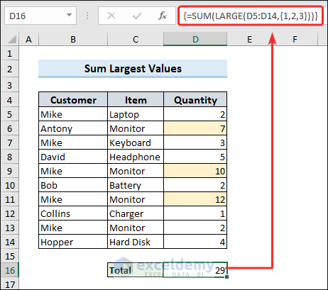
Example 10 – Sum a Range with Text Values and Errors in Excel

• Use the following formula to ignore non-number values.

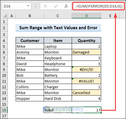
Frequently Asked Questions

What is the sum range?

The sum range refers to the range of cells that you want to add together. It is the set of cells that you specify as the input for the function to calculate the sum.

What is subtotal in Excel?

In Excel, the SUBTOTAL function is used to calculate various types of subtotals within a range of data. The SUBTOTAL function is particularly useful when working with filtered data or when you want to calculate subtotals for specific sections within a larger dataset.

Key Takeaways from the Article

• SUMIF and SUMIFS functions are used to sum cells based on condition.
• The SUBTOTAL function is used to find the sum of filtered cells.
• AutoSum feature inserts the SUM function to calculate the sum.
• Texts and errors can be handled with the IFERROR function.

Sum in Excel: Knowledge Hub

<< Go Back to How to Calculate in Excel | Learn Excel