In this article, you will learn how to use absolute, relative, and mixed cell references.
We’ll use a sample dataset for Products and Sales, in which we have individually referred to cells and summed them up.
⏷What is Cell Reference?
⏷How to Create or Change a Cell Reference
⏵A Simple Reference
⏵Reference a Cell Range
⏵Cell Reference in a Function
⏵Reference Text in Another Cell
⏵Use Cell Reference in a Formula Using Worksheet Name
⏵Cell Reference Using OFFSET Function
⏷Clicking Cells to Refer
⏷Types of Cell References
⏵Relative Cell Reference & Its Application
⏵Absolute Cell Reference & Its Application
⏵Mixed Cell Reference & Its Application
⏷Switch Among Relative, Absolute, and Mixed References
⏷Difference Between Absolute, and Relative Cell Reference
⏷Refer Entire Row or Column
⏷Refer Entire Column Except for First Few Rows
⏷Variable Row & Column Number As Cell Reference
⏷Cell Reference to Refer Another Worksheet or Workbook
⏷Difference Between A1 and R1C1 Reference Style
⏷Named Range to Refer Cells
⏷Circular Reference in Excel
⏷3D Reference in Excel
What Is a Cell Reference?
A cell reference in Excel identifies the location of a specific cell as indicated by its column letter and row number. It is crucial in creating formulas, and there are three types:
- Absolute ($) references stay fixed when copied.
- Relative references adjust based on the new location.
- Mixed references have a combination of absolute and relative components.
Cell references create dynamic formulas that can be replicated and adapted, allowing for efficient data analysis and manipulation.
How to Create or Change a Cell Reference
Example 1 – A Simple Reference
A simple reference in Excel involves pointing to the content of a single cell using its column letter and row number (e.g., C6).
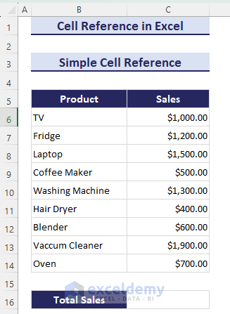
In this section, we have used Product and corresponding Sales data. Here we will use individual product sales values from C6 to C14 and sum them up individually.
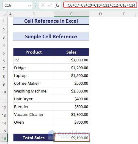
- We have used the formula below in the C16 cell:
=C6+C7+C8+C9+C10+C11+C12+C13+C14
Example 2 – Reference a Cell Range
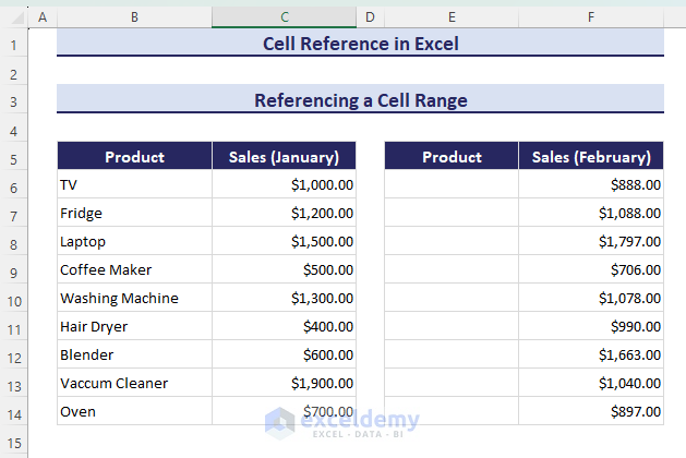
We have Products and Sales for two different months, January and February. As the product names are the same for both months, we can refer to the cell values of January in February.
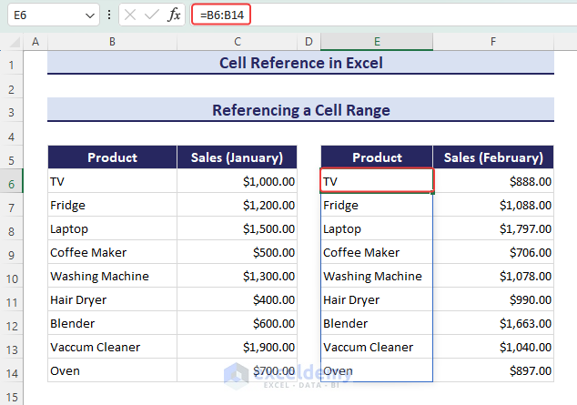
- We will referenced a cell range B6 to B14 in the E6.
- We have used the formula below in the E6 cell:
=B6:B14
Example 3 – Cell Reference in a Function
To find the Total Sales from a dataset with Product and Sales information, we will add up all the sales values in the dataset.
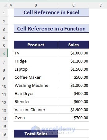
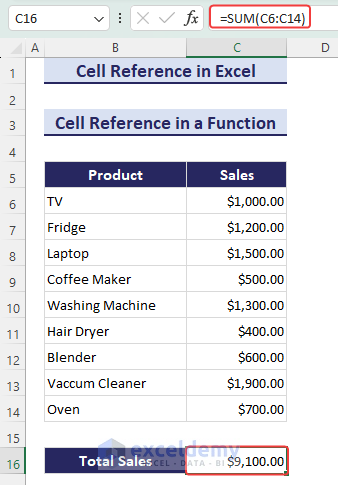
- We have used the SUM function in the formula below using the cell reference C6:C14:
=SUM(C6:C14)
which would replace the more convoluted list:
=SUM(C6,C7,C8,C9,C10,C11,C12,C13,C14)
Example 4 – Reference Text in Another Cell
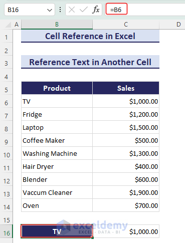
In this section, we have a dataset of Product and Sales values. The cell C16 is fetching a sales value based on the value of cell B16. We have to refer to the Product to find the corresponding sales value.
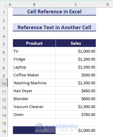
- We used the formula below in the B16 cell:
=B6
Example 5 – Use a Cell Reference in a Formula with a Worksheet Name
For example, =Sheet2!A1 refers to cell A1 in the Sheet2 worksheet. This is one of the few ways you can cross-reference between worksheets.
We are going to find the total sales when sales data is in another worksheet Jan.
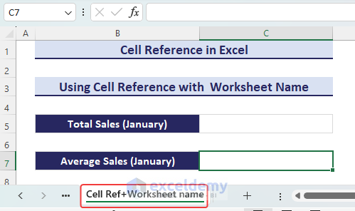
- We have used this formula in the C5 cell.
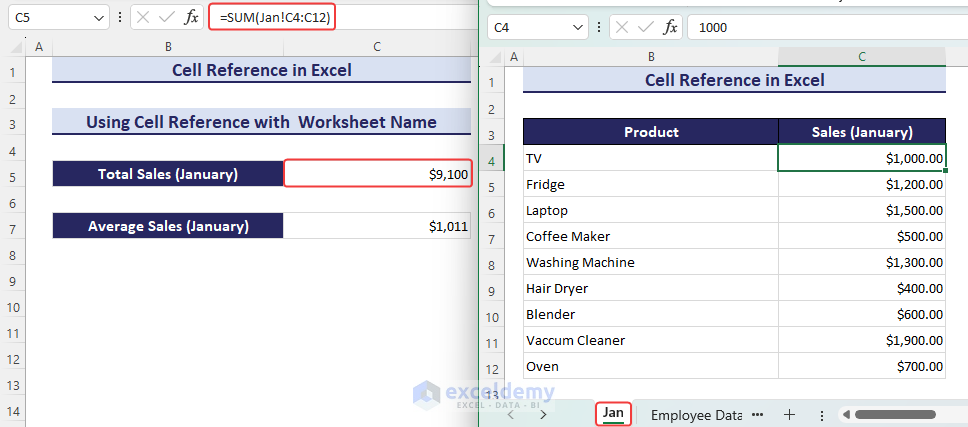
=SUM(Jan!C4:C12)
The formula =SUM(Jan!C4:C12) in cell C5 of the current worksheet calculates the sum of values in the range C4 to C12 of another worksheet named Jan.
- We have used the Jan worksheet to get the total sales.
Example 6 – Cell Reference Using the OFFSET Function
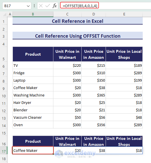
We have a dataset of prices of different products in different shops. We will extract the whole row.

- We have used the formula below in cell B17:
=OFFSET(B5,4,0,1,4)
Example 7 – Clicking on Cells to Refer to Them
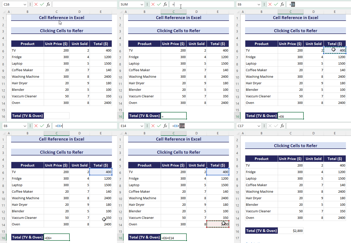
Let’s sum the sales of TV and Oven.
- Clicking on the result cell.
- Input the = sign to insert the formula in the formula bar.
- Select the cells you want to refer to.
- Click on E6, type +, and click on E14 to calculate the total sales for TV and Oven.
- Press Enter.
Types of Cell References and How to Use Them
Type 1 – Relative Cell Reference
A relative cell reference adjusts its position when copied to a new location. It refers to a cell’s position relative to the one containing the formula.
For instance, when multiplying B6*C6 in a cell and dragging the Fill handle down, the formula for subsequent rows will multiply B7*C7, B8*C8, and so on.
Pros:
- Ease of Copying: Simplifies copying formulas to different cells.
- Dynamic Formulas: Formulas adjust to new locations, making them versatile.
- Efficiency in Maintenance: Changes in one cell often apply universally when copied, reducing manual effort.
- Consistency in Patterns: Formulas with relative references follow consistent patterns, aiding readability.
Cons:
- Potential Error Risk: If not used carefully, relative references might lead to errors when formulas are copied.
- Less Control Over Specific References: You can’t lock specific cells in a formula to prevent them from changing when copied.
- Complexity in Special Cases: In certain complex spreadsheet scenarios, relative references might not be the ideal choice.
- Dependency on Cell Layout: Formulas depend on the layout of cells, so if cells are moved, the results might change unexpectedly.
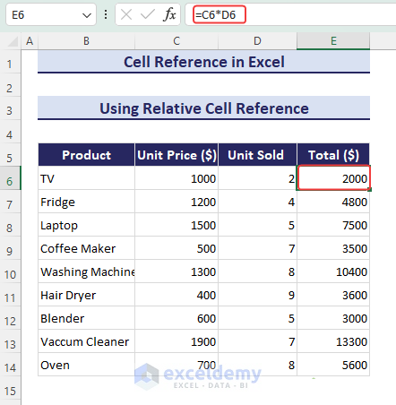
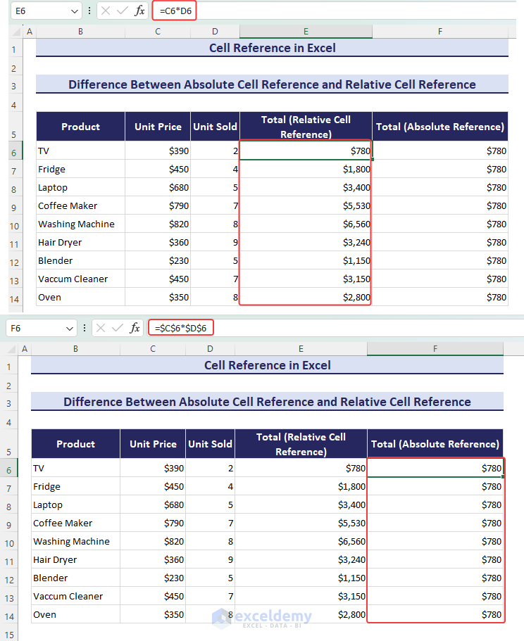
We have a dataset for the Unit Price of some products and the number of Unit Sold. We have multiplied C6 and D6. When we drag and drop the Fill Handle, we will get respective multiplications such as C7*D7, C8* D8, and so on.
- The formula is given below:
=C6*D6
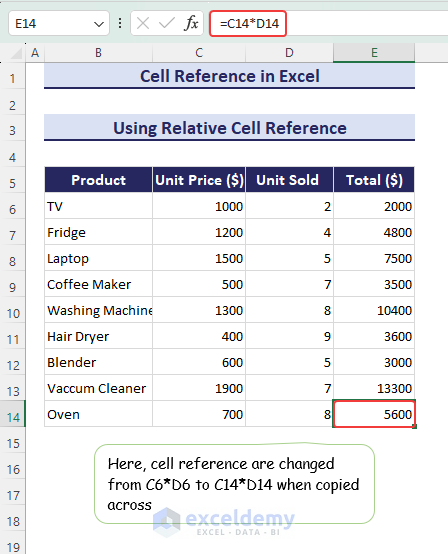
- We can see the last cell reference is C14*D14. The cell reference for the row numbers in both values has changed by dragging the fill handle down.
Type 2 – Absolute Cell Reference
An absolute cell reference does not change the referred cell when you drag down the Fill Handle or copy the formula. If you put $C$6 as an absolute cell reference, the C6 will be constant throughout the cells after you drag the Fill Handle.
Pros:
- Control Over Specific References: Allows you to “lock” specific cells in a formula, preventing them from changing when copied.
- Stability in Formulas: References remain fixed, providing stability in calculations even when formulas are copied.
- Less Error-Prone: Reduces the risk of errors caused by unexpected changes in references during copying.
- Useful in Fixed Data Scenarios: Ideal for scenarios where certain values or constants need to stay constant across multiple calculations.
Cons:
- Less Dynamic: Formulas can be less dynamic and adaptable to changes in cell locations.
- Increased Complexity: Involves the use of dollar signs ($) which may add complexity, especially for beginners.
- More Effort in Formula Maintenance: Changing specific references requires a manual adjustment in each formula.
- Potential for Redundancy: In some cases, absolute references might lead to redundant formulas when applied across different cells.
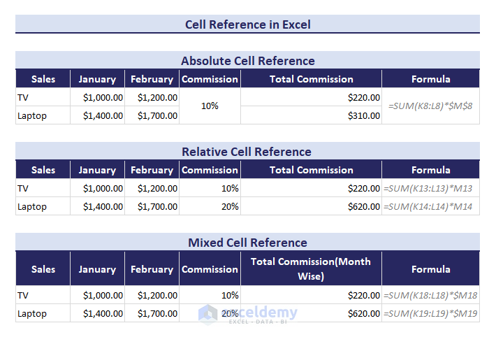
We have used the commission percentage as an absolute cell reference in the dataset for the Products. We have to write the formula in the F8 cell. Commission, $C$5, is an absolute cell reference and the C5 cell will be fixed:
=E8*$C$5
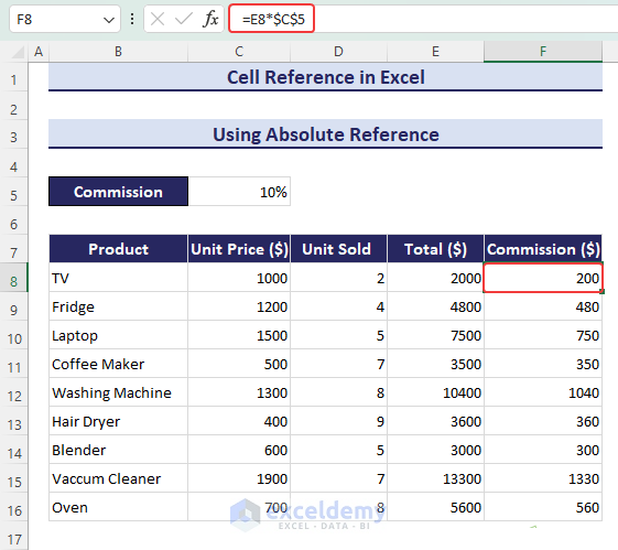
- Unlike a relative cell reference, we can see that the first argument has changed but C5 did not change its position according to E.
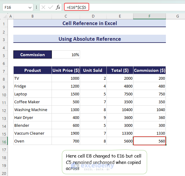
Type 3 – Mixed Cell Reference
A mixed cell reference is a blend of fixed (absolute) and relative references. For example, with $C6, column C stays constant as you drag horizontally, while C$6 keeps row 6 fixed when dragged vertically. It’s a handy way to control references partially in formulas.
Pros:
- Flexibility in Locking: Allows for a mix of absolute and relative references, providing flexibility in controlling certain aspects of the formula.
- Balanced Adaptability: Offers a balance between the adaptability of relative references and the stability of absolute references.
- Efficient Maintenance: Easier formula maintenance compared to absolute references, as some references can adapt while others remain fixed.
- Useful in Many Scenarios: Well-suited for scenarios where some elements of the formula need to change dynamically while others stay constant.
Cons:
- Potential for Confusion: Beginners might find the mix of absolute and relative references confusing.
- Complexity in Formulas: Depending on the mix used, formulas can still become complex, especially in intricate spreadsheet models.
- Careful Management Required: Requires careful management to ensure that the mix of references aligns with the desired behavior of the formula.
- Not Universally Applicable: Might not be the best choice in all scenarios.
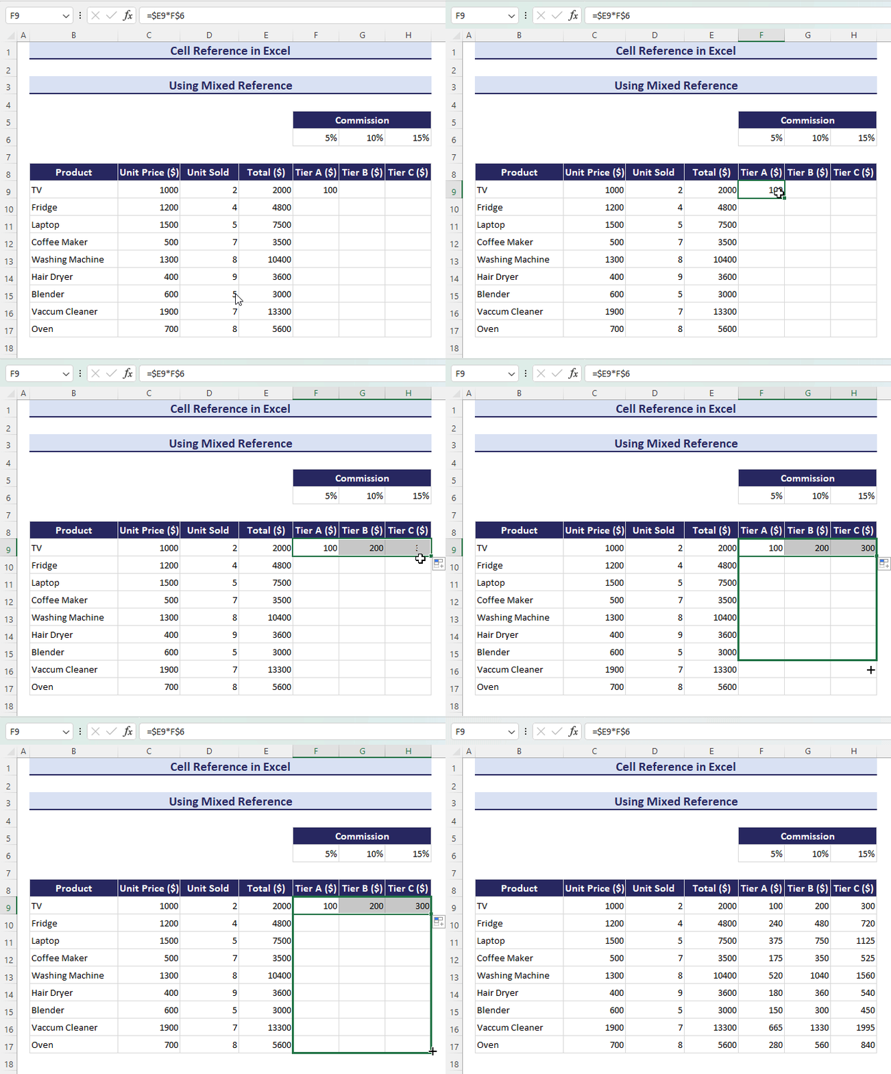
We will use three different types of commission in three different tiers. So, we have to make some rows absolute and some columns relative.
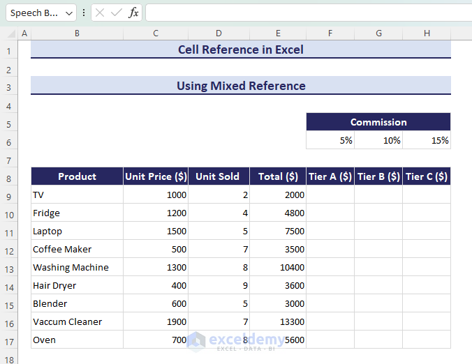
- Use the formula below in F9:
=$E9*F$6
Here, column E will not change (so we lock the product sales reference) and row 6 will not change (since it contains the commission values) because the $ sign is given before them.
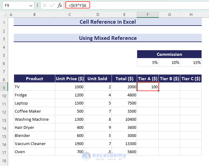
- Fill the rest of the values by dragging the Fill Handle right, then down.
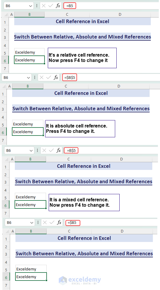
How to Switch Between Relative, Absolute, and Mixed References in Excel
To switch between references, press F4 while referencing a cell. It will change your cells to relative, absolute, and mixed references in the following order:
- Relative
- Absolute
- Fixed column
- Fixed row
- Back to relative
Differences Between Absolute and Relative Cell References in Excel
We have calculated the Total using both relative cell reference and absolute cell reference. When we use a relative cell reference, the total revenue will change respectively. But when we use an absolute cell reference, the total revenue will not change for the other rows.
How to Reference an Entire Row or Column in Excel?
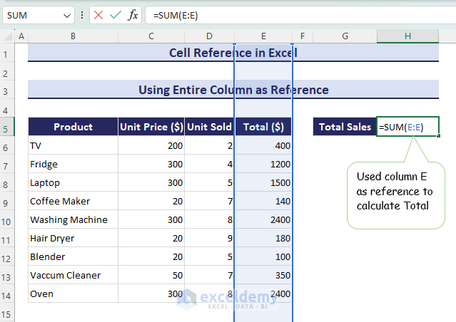
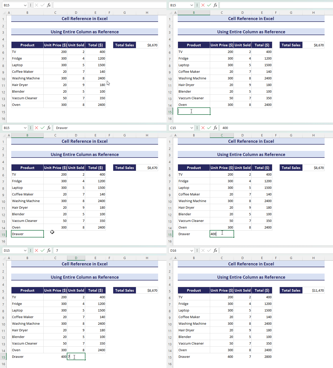
- To use the entire column E as a reference, we have used the formula below in G cell:
=SUM(E:E)
- We get the total in cell H5.
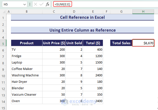
- When you add new data, it will automatically update the total sales.
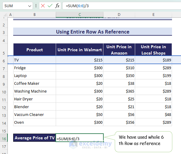
We’ll find the average price of a TV by referencing an entire row.
- We have used the formula below in cell C16 to reference the entire sixth row:
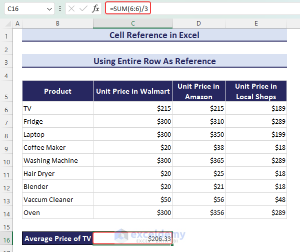
=SUM(6:6)/3
- The output uses the entire 6th row as a reference. When you change the prices in this row, the average price will change automatically.
How to Reference an Entire Column Except for First Few Rows in Excel
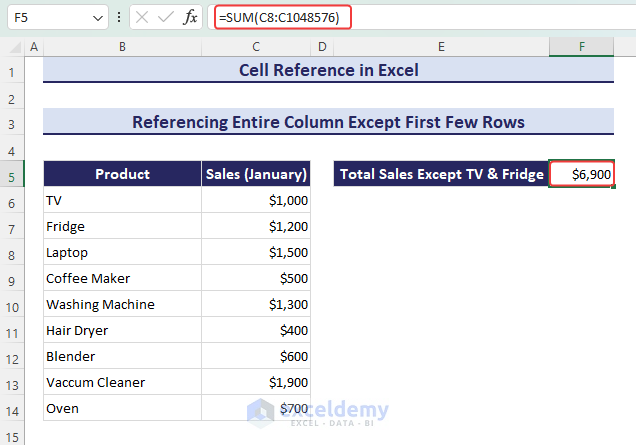
In this section, we have used the dataset of Product and Sales. But, we will ignore some rows. Here we reference from row C8 to C1048576 (max value for row numbers), leaving out C1 to C7.
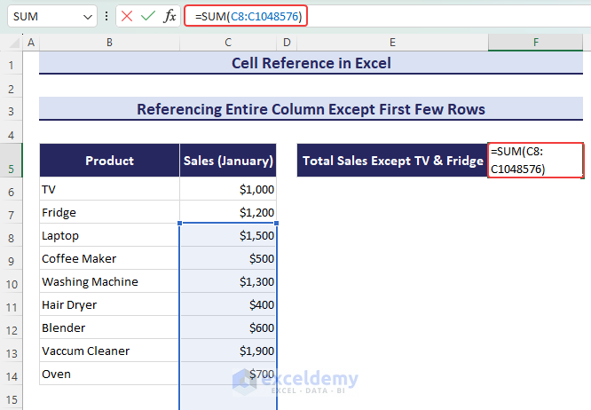
- We have used the formula below in the F5 cell:
=SUM(C8:C1048576)
How to Use Variable Row and Column Numbers as a Cell Reference in Excel
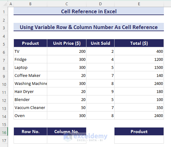
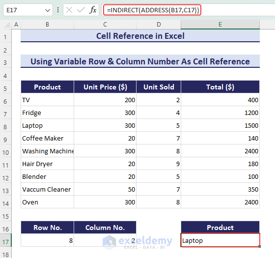
We will create a user-input model where you can select any row and column number in two separate cells and fetch the value of the corresponding cell.
- We used the formula below in cell E17:
=INDIRECT(ADDRESS(B17,C17))
How to Use a Cell Reference to Refer to Another Worksheet or Workbook in Excel
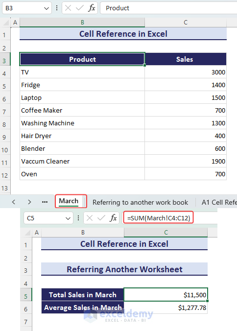
We have used the formula below to refer to another worksheet March in the present worksheet:
=SUM(March!C4:C12)
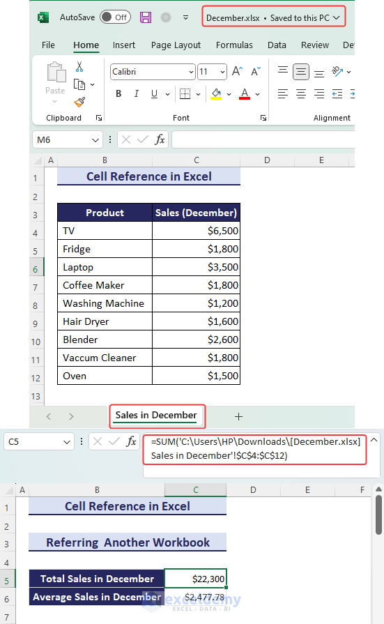
We have another workbook named December.xlsx and from the Sales in December worksheet, we want to get the total sales and average sales.
- We used the formula below to refer to another workbook:
SUM('C:\Users\HP\Downloads\[December.xlsx] Sales in December'!$C$4:$C$12)
What Is the Difference Between the A1 and R1C1 Reference Styles in Excel?
There are two styles of cell references: A1 and R1C1.
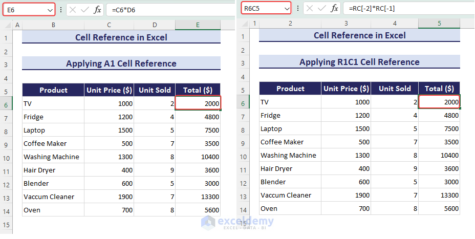
The A1 reference style identifies cells by letters and numbers (e.g., A1). The R1C1 reference style uses row and column offsets from the active cell (e.g., R2C3 means two rows down and three columns to the right of the active cell).
We will calculate the Total price for the below dataset and show the formula using both reference styles.
- The formula with A1 reference style is as follows:
=C6*D6
C6 refers to the cell in column C and 6th
D6 refers to the cell in the second column D and 6th
- The formula with R1C1 reference style is as follows:
=RC[-2]*RC[-1]
RC[-2] refers to two columns to the left of the current column, and RC[-1] refers to one column to the left.
If you need to go one row up while staying in the same column, you’d put R[-1]C.
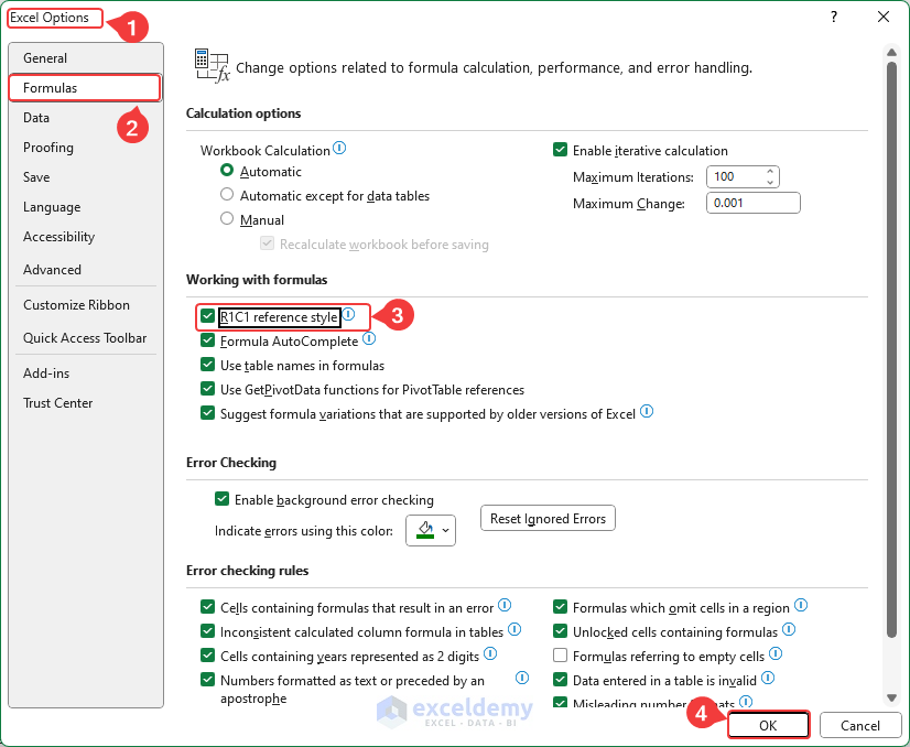
- To enable the R1C1 reference style, press Alt + F + T, choose Formulas, check the R1C1 reference style, and press OK.
How to Use a Named Range to Refer to Cells in Excel
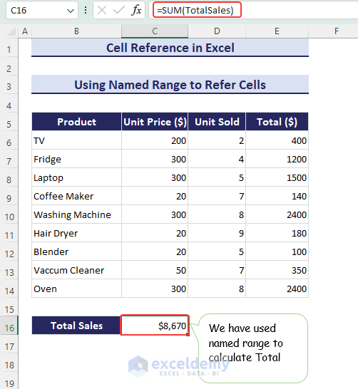
- We named the range E6 to E14 as TotalSales.
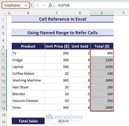
- We have used the defined name in the SUM formula to get total sales:
=SUM(TotalSales)
Read More: Excel Use Cell Value as Worksheet Name in Formula Reference
What Is a Circular Reference in Excel?
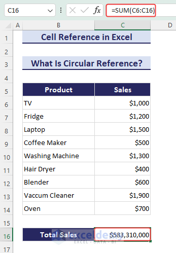
A circular reference in Excel happens when a cell’s formula refers to itself or creates a loop with other cells, causing calculation issues.
Here C16 refers to itself. Every time you open the worksheet, it will add the previous data and you will get an ever-increasing sum.
- For a new Excel workbook, it may return zero, too:
=SUM(C6:C16)
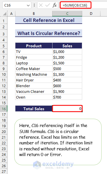
- When you create a circular reference, you will usually get a warning.

How to Use a 3D Reference in Excel
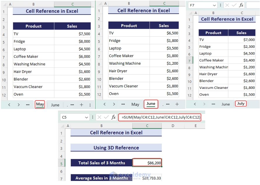
A 3D reference in Excel is a way to combine information from the same cell or range of cells across multiple sheets in a workbook. It’s like looking at the data from different sheets all at once.
We have extracted the corresponding sales columns of May, June, July worksheets and summed them up by using the formula below:
=SUM(May!C4:C12,June!C4:C12,July!C4:C12)
Download the Practice Workbook
Cell Reference in Excel: Knowledge Hub
<< Go Back to Excel Formulas | Learn Excel
Get FREE Advanced Excel Exercises with Solutions!
