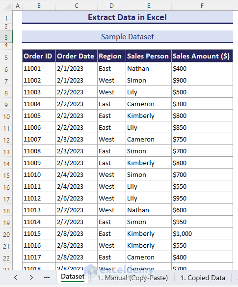
This is a dataset of Order Management.
And this is our sample dataset.
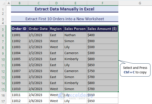
Method 1 – Extracting Data from Excel Manually
- Select the B5:F15 range and press Ctrl + C to copy the first 10 orders.
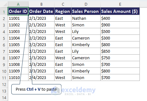
- Go to the new worksheet and paste them by pressing Ctrl + V.
Data is moved into a new worksheet.
Method 2 – Extracting Filtered Data from an Excel Sheet
2.1. Using the Basic Filter Tool to Extract Filtered Data
- Select the B5:F5 range.
- Go to Home => Editing => Sort & Filter => Filter.
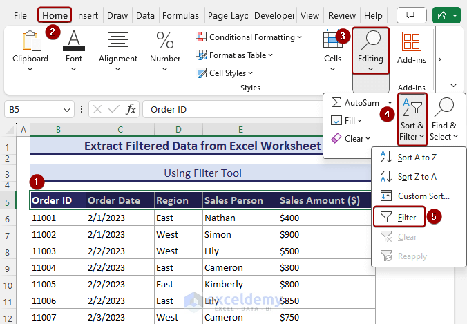
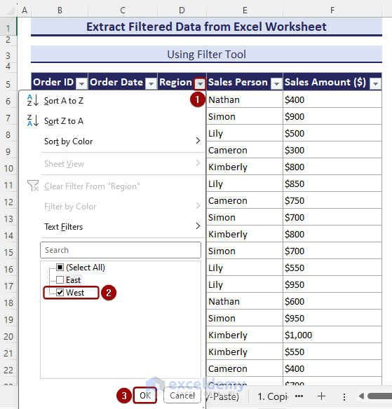
- Select Filter drop-down box => Check West Region=> OK.
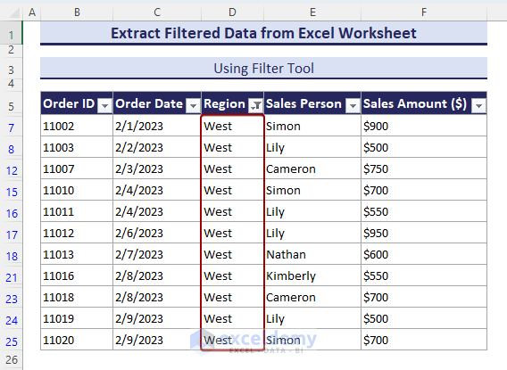
Data of the west region is displayed.
2.2. Using the Excel FILTER Function to Extract Data Based on Criteria
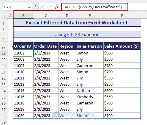
- Insert the following FILTER formula in B28.
=FILTER(B6:F25,D6:D25="west")All information on the “West” region will be displayed in array format.
2.3. Using an Advanced Filter to Extract Data Based on Multiple Criteria
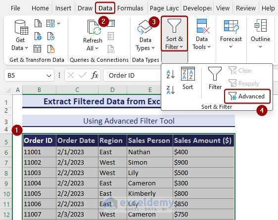
- Select the entire data range.
- Click Data => Sort & Filter => Advanced.
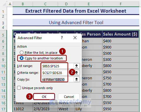
- In Action, choose Copy to another location.
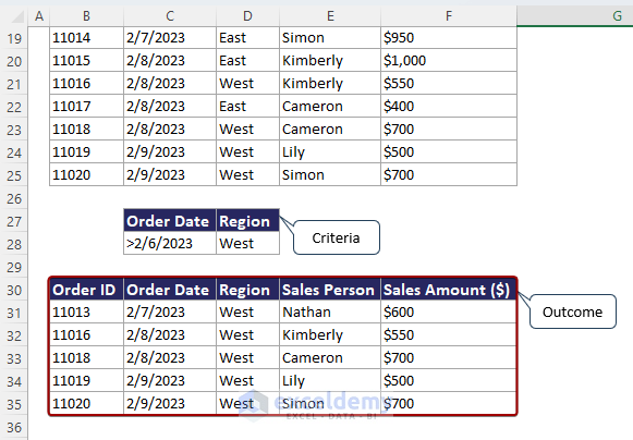
- Select List range $B$5:$F$25, Criteria range $C$27:$D$28 and output location $B$30.
All data of the west region with order dates from 2/6/2023 onward will be displayed.
Method 3 – Extracting Specific Data from a Column in Excel
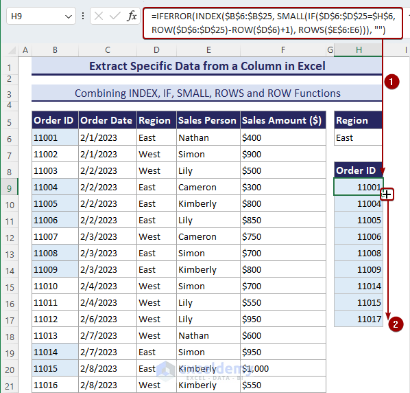
- Enter the following formula in H9 and press Enter.
=IFERROR(INDEX($B$6:$B$25, SMALL(IF($D$6:$D$25=$H$6, ROW($D$6:$D$25)-ROW($D$6)+1), ROWS($E$6:E6))), "")- Order Id 11001 from the East region will be displayed. Drag the Fill Handle tool see all Order IDs.
Method 4 – Extracting Data from an Excel Cell
- Enter the following formula in E6 and drag the Fill Handle tool.
=LEFT(B6,FIND(" ",B6)-1)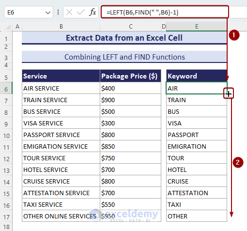
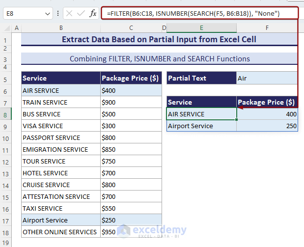
Method 5 – Extracting Data Based on Partial Input from a Cell
- Enter this FILTER-ISNUMBER-SEARCH formula in E8.
=FILTER(B6:C18, ISNUMBER(SEARCH(F5, B6:B18)), "None")All information containing the text “Air” will be displayed in array format.
Method 6 – Using an Excel Formula to Extract Data Based on the Lookup Value
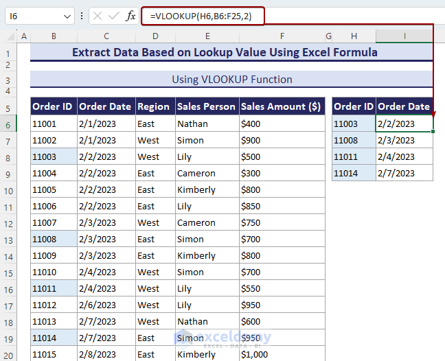
6.1. Using the VLOOKUP Function
- Enter the following formula in I6.
=VLOOKUP(H6,B6:F25,2)- Drag the Fill Handle to see the Order Dates for each Order ID.
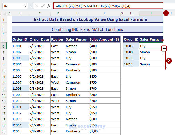
6.2. INDEX-MATCH Formula
- Enter the following formula in I6 to see the Sales Person (Lily).
=INDEX($B$6:$F$25,MATCH(H6,$B$6:$B$25,0),4)- Drag the Fill Handle to see the Order Dates for each Order ID.
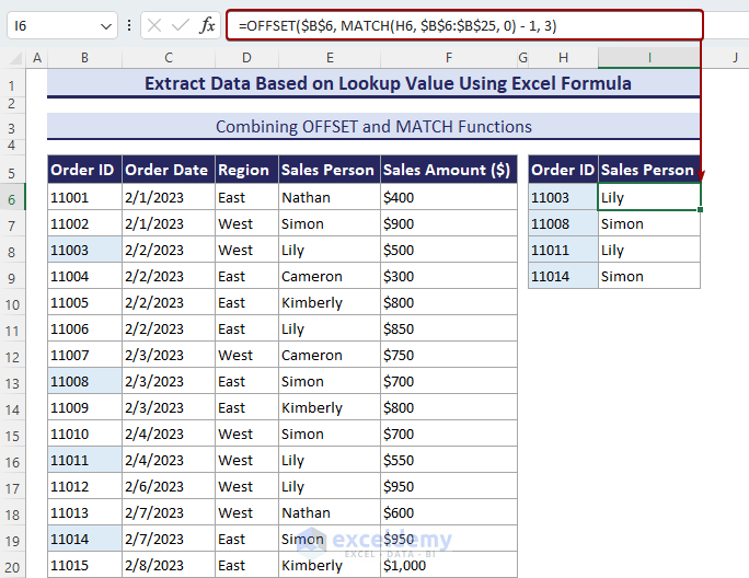
6.3. Using OFFSET and MATCH Function
- Enter the following formula in I6 to see the Sales Person (Lily) .
=OFFSET($B$6, MATCH(H6, $B$6:$B$25, 0) - 1, 3)- Drag the Fill Handle to see the Order Dates for each Order ID.
Method 7. Pulling Data from a Worksheet Using the Data Consolidate Tool
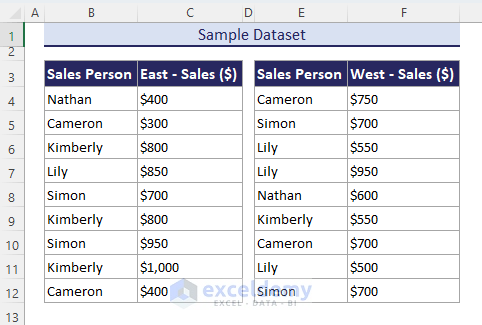
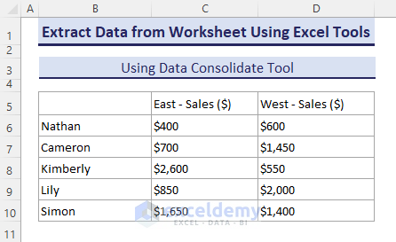
There are two datasets in a worksheet.
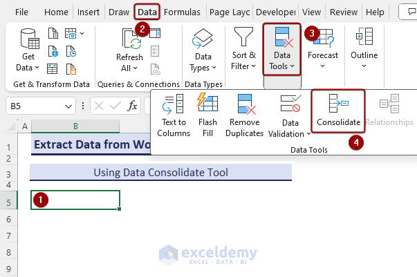
- Select B5.
- Go to Data => Data Tools => Consolidate.
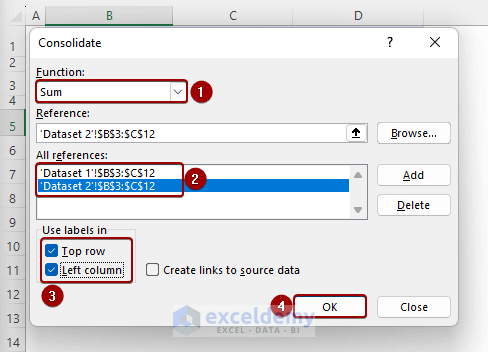
- In Function, choose Sum.
- Add references from Dataset 2.
- In Use labels in, check Top row and Left column.
- Click OK.
Data is displayed together in the dataset.
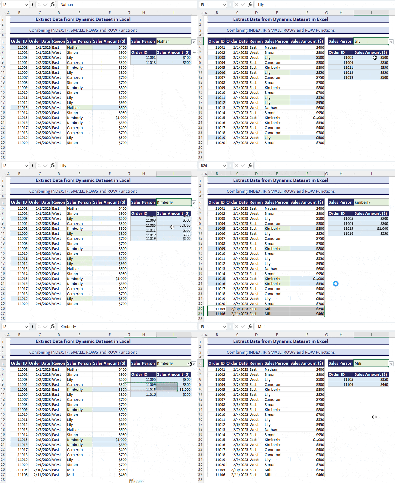
Method 8 – Extracting Information from a Dynamic Dataset in Excel
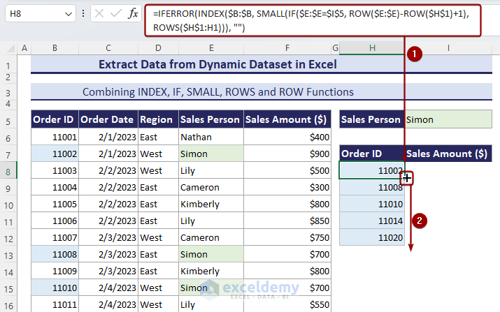
- Enter the formula below in E8.
=IFERROR(INDEX($B:$B, SMALL(IF($E:$E=$I$5, ROW($E:$E)-ROW($H$1)+1), ROWS($H$1:H1))), "")- Drag the Fill Handle across the cells you want to fill.
- Enter the following formula in I8.
=IFERROR(INDEX($F:$F, SMALL(IF($E:$E=$I$5, ROW($E:$E)-ROW($H$1)+1), ROWS($H$1:H1))), "")The total of 5 Order IDs and Sales Amount ($) for Simon will be displayed.
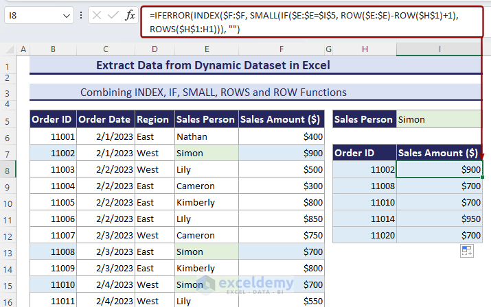
- Information was added to Sales Person list. By selecting Mili from the drop-down list, you will also be able to extract data.

Method 9 – Using a Pivot Table to Extract Data in Excel
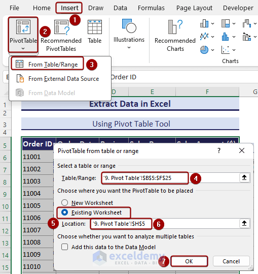
- To convert a range into Pivot Table, click Insert => PivotTable => From Table/Range.
- In the PivotTable from table or range dialog box, choose Table/Range range => Pivot table location => OK.
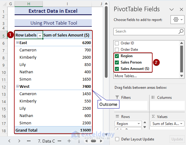
- Check Region, Sales Person, and Sales Amount ($) in PivotTable Fields.
- The Sum of Sales for each person in separate regions will be displayed.
Method 10. Applying a VBA Macro to Extract Data
- Enter the following VBA code in the Module and save the Macro.
Sub Extract_Data_from_Excel()
'Developed by MD Tanvir Rahman, ExcelDemy
Dim Inp As Range, Cri As Range, Out As Range
Dim out_row As Long
Set Inp = Application.InputBox("Select input range:", Type:=8)
Set Cri = Application.InputBox("Select Sales Person:", Type:=8)
Set Out = Application.InputBox("Select Output Location:", Type:=8)
out_row = 1
For i = 1 To Inp.Rows.Count
    If Inp.Cells(i, 4) = Cri.Value Then
        Out.Cells(out_row, 1) = Inp.Cells(i, 1).Value
        Out.Cells(out_row, 2) = Inp.Cells(i, 5).Value
        out_row = out_row + 1
    Else
    End If
Next i
End Sub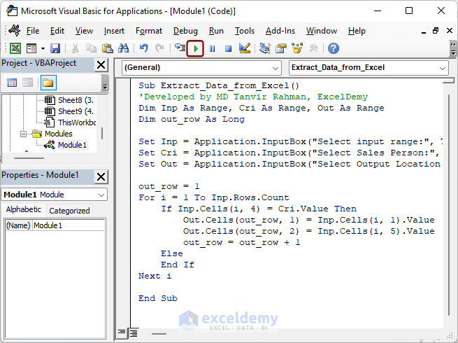
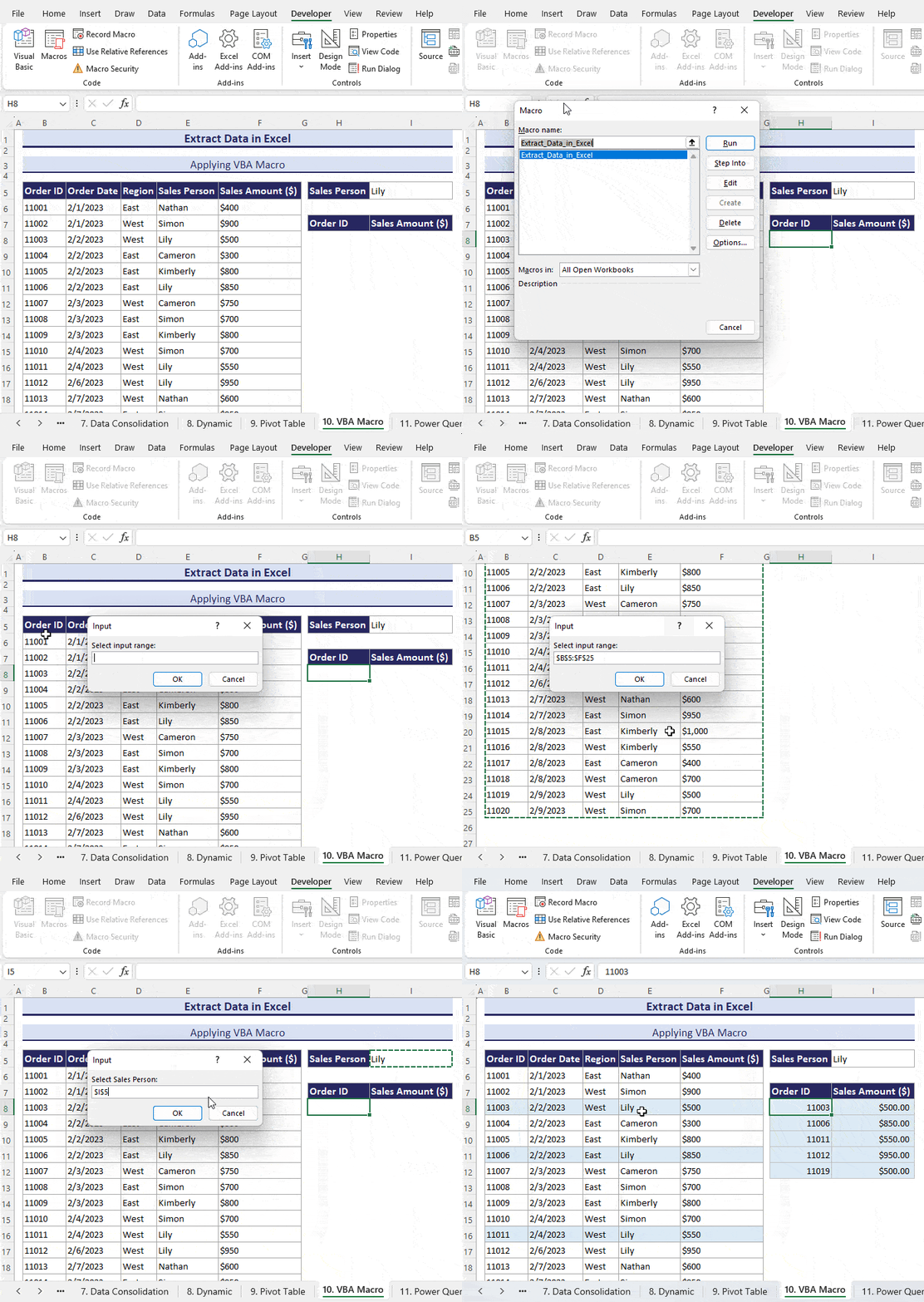
- Select Developer => Macros => Extract_Data_from_Excel => Run.
- Select input range, criteria and output range.
- The Order ID and Sales Amount ($) for Lily will be displayed.
Method 11. Applying the Excel Power Query to Extract Data
The following dataset is a plain text file.
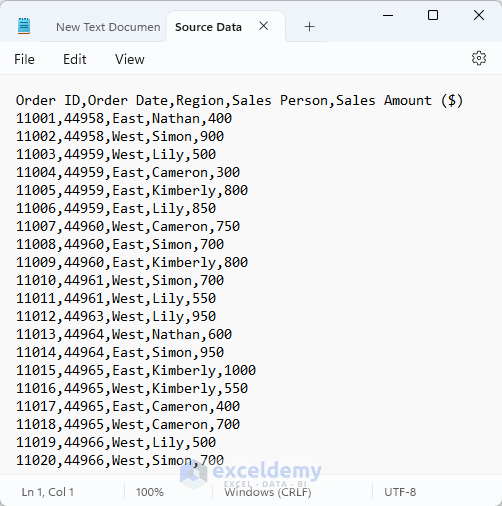
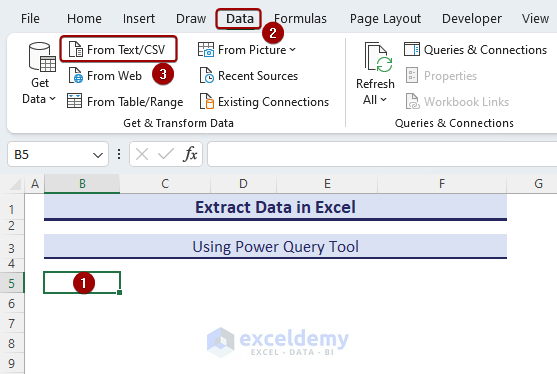
- To import data from a plain text (.txt) file, select B5 and click Data => From Text/CSV.
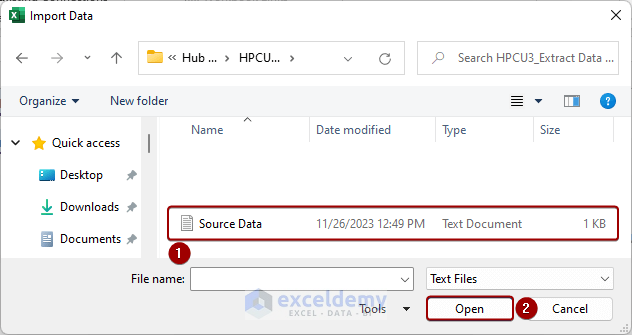
- Select the Source Data file => Open.
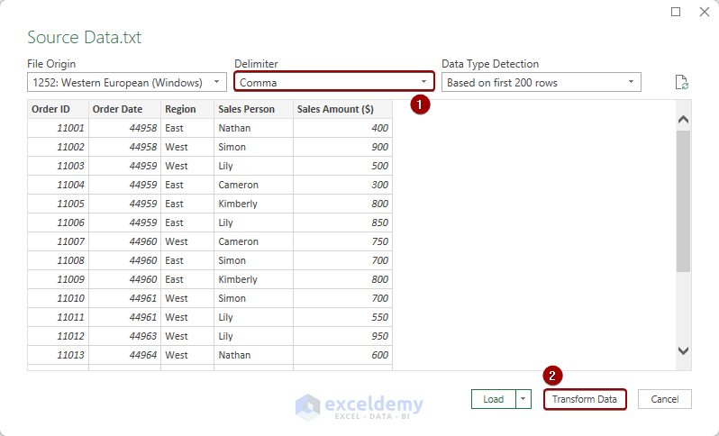
- Select Comma Delimiter => Transform Data.
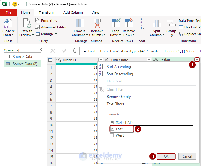
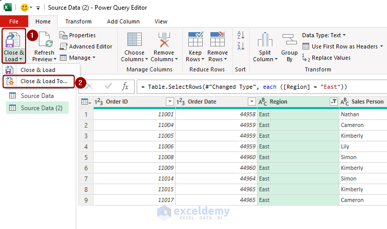
- Click the Region drop-down menu => Check East => OK.
- Select Close & Load drop-down => Close & Load To.
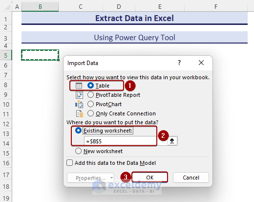
- In the Import Data dialog box, select Table => Existing worksheet => $B$5 => OK.
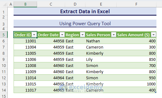
All data containing the East region is displayed in the Excel worksheet.
Method 12 – How to Extract a Specific Number of Characters from a Cell
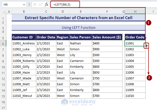
- Enter the following formula in H6 to see the Order Code.
=LEFT(B6,5)- Drag the Fill Handle across the cells you want to fill.
Method 13 – How to Extract Month and Day from Date in Excel
- Enter the following formula in F6 to see the month.
=TEXT($C6,"mmmm")- Drag the Fill Handle across the cells you want to fill.
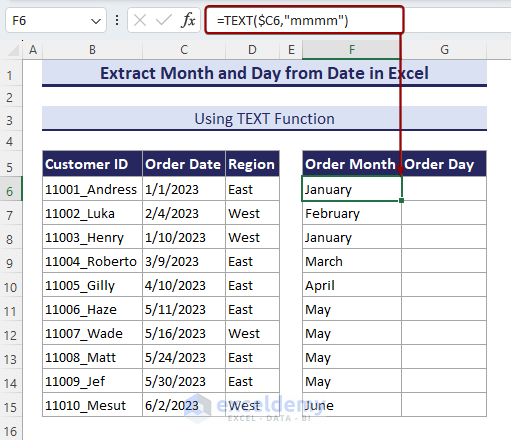
- Enter the following formula in G6 to see the order day.
=TEXT($C6,"dddd")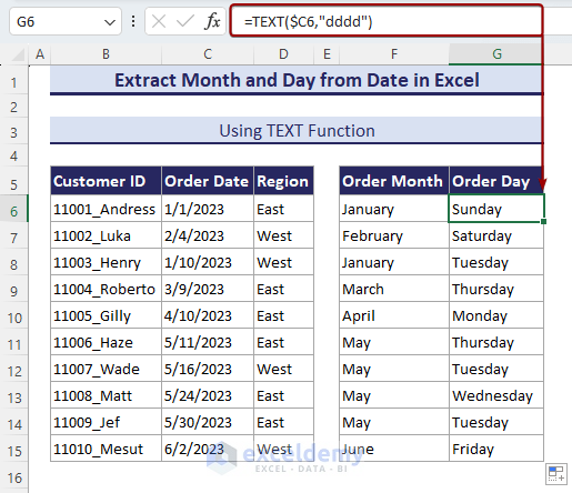
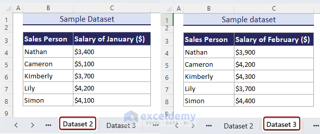
Method 14 – How to Extract the Same Cell from Multiple Sheets into a Master Column in Excel
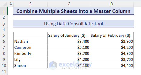
There are two datasets: Dataset 2 and Dataset 3.
- In Function, select Sum.
- Add references from Dataset 2 and Dataset 3.
- In Use labels in, check Top row and Left column.
- Click OK.
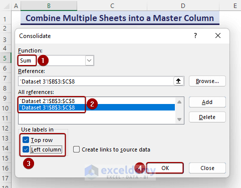
Data from multiple worksheets is combined.
Download Practice Workbook
Download the Practice workbook and practice.
Extract Data Excel: Knowledge Hub
- Excel Formula to Get First 3 Characters from a Cell
- Extract Data from a List Using Excel Formula
- Extract Month from Date in Excel
- Extract Year from Date in Excel
- Pull Data From Another Sheet Based on Criteria in Excel
- Get Data from Another Sheet Based on Cell Value in Excel
- Extract Filtered Data in Excel to Another Sheet
- Pull Values from Another Worksheet in Excel
- Pull Data from Multiple Worksheets in Excel
- Extract Data from One Sheet to Another Using VBA in Excel
- Pull Data from Multiple Worksheets in Excel VBA
- Excel Macro: Extract Data from Multiple Excel Files
<< Go Back To Learn Excel
Get FREE Advanced Excel Exercises with Solutions!

