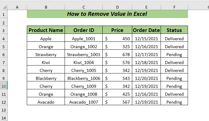
The below dataset has 5 columns: Product Name, Order ID, Price, Order Date, and Status.
Method 1 – Using a Keyboard Shortcut
Steps:
- Select any cell or cell range from where you want to remove the value. I selected the cell F7
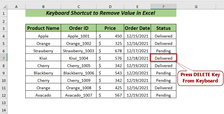
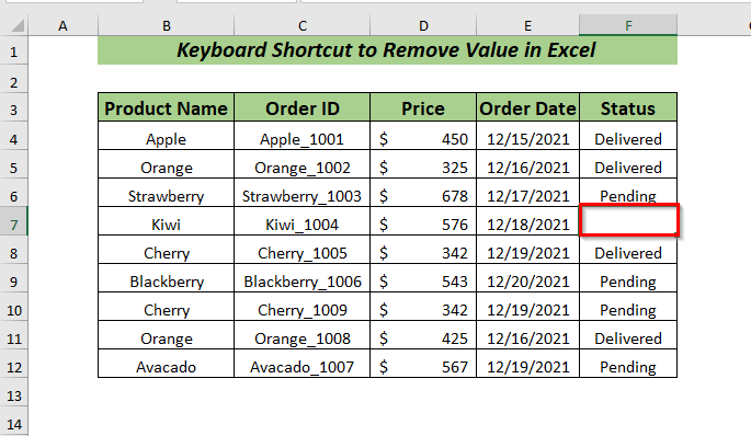
- Press DELETE and the value will be removed from the selected cell.
Read More: How to Remove Numbers from a Cell in Excel
Method 2 – Using Sort with Right Click
Steps:
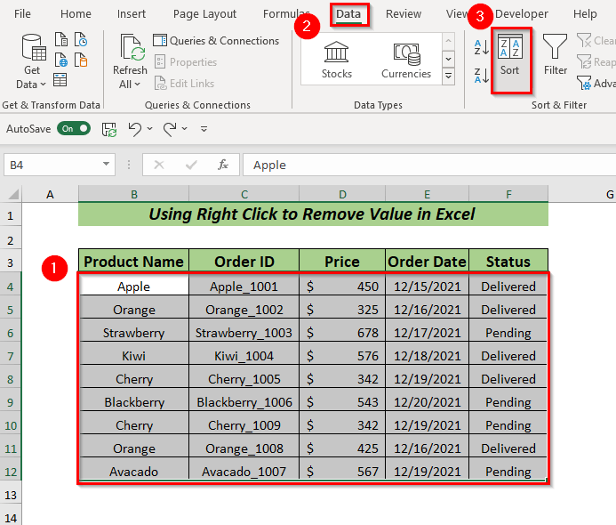
- Select the cell range to apply Sort. I selected the cell range B4:F12
- Open the Data tab >> Select Sort
- A dialog box will pop up. In Sort by, I selected Status.
- Click OK.
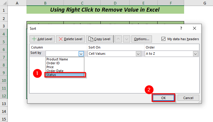
Here, Sort is applied, and all the values are sorted in A to Z Order according to the Status column value.
Suppose you want to remove the values of those products that have been delivered.
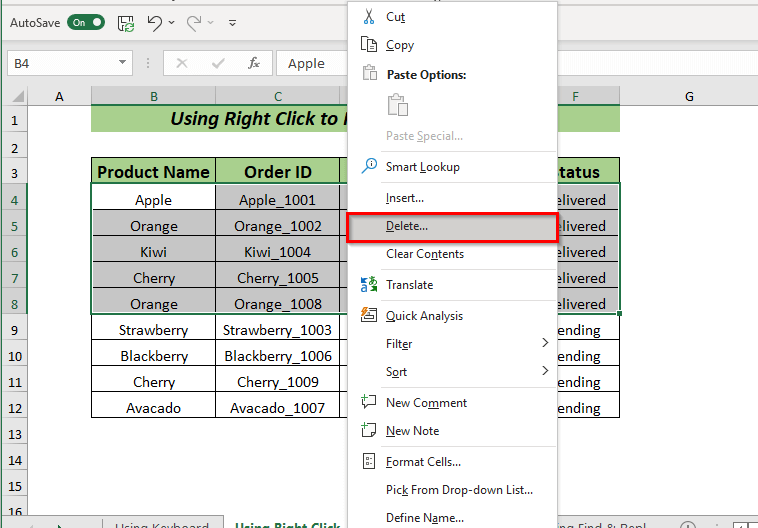
- Select the delivered product values and right-click.
- From the context menu, select Delete.
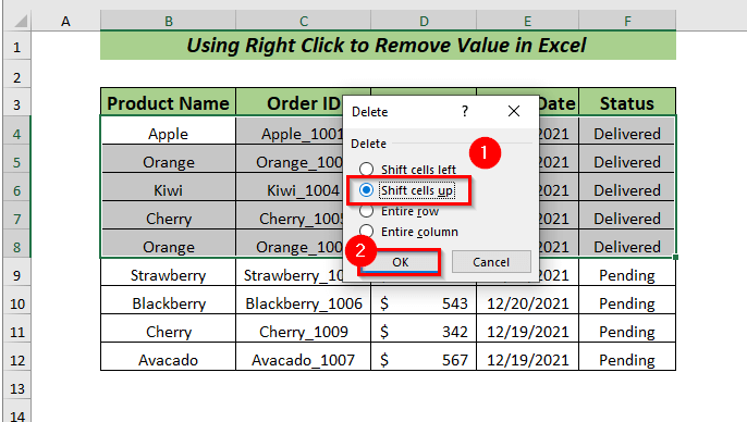
- A dialog box for the Delete option will appear. I selected the Shift cells up option.
- Click OK.
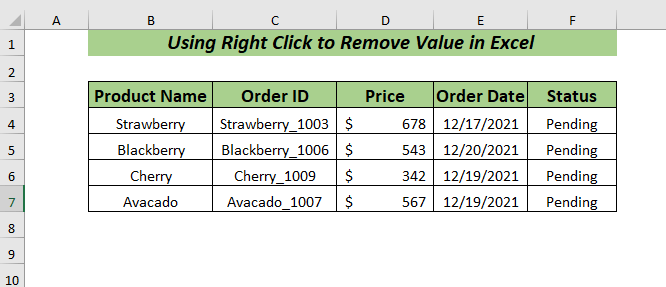
The selected values are removed from the sheet.
Method 3 – Using Ribbon with Sort
Steps:
- Select the cell range to apply Sort. I selected the cell range B4:F12
- Open the Data tab >> Select Sort
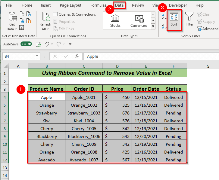
- A dialog box will pop up. In Sort by, I selected Status.
- Click OK.
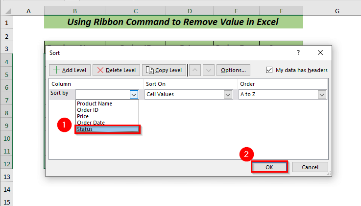
Here, Sort is applied, and all the values are sorted in A to Z Order according to the Status column value.
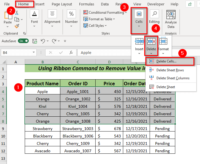
- To remove the value of your choice, select the cell or cell range. I selected the cell range B4:F8.
- Open the Home tab >> go to the Cells group >> from the Delete >> select Delete Cells
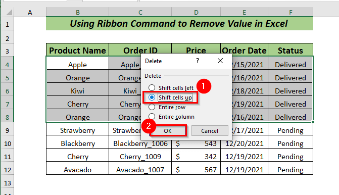
- A dialog box for the Delete option will pop up. I selected the Shift cells up option.
- Click OK.
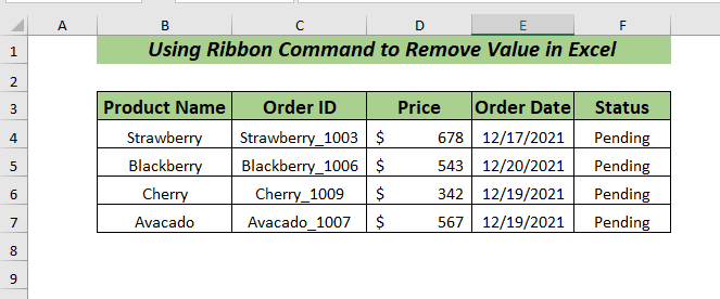
All the selected values are removed.
Read More: How to Remove Outliers in Excel
Method 4 – Using Find & Replace to Remove Value
Steps:
- Open the Home tab >> go to Editing group >> from Find & Select >> select Replace
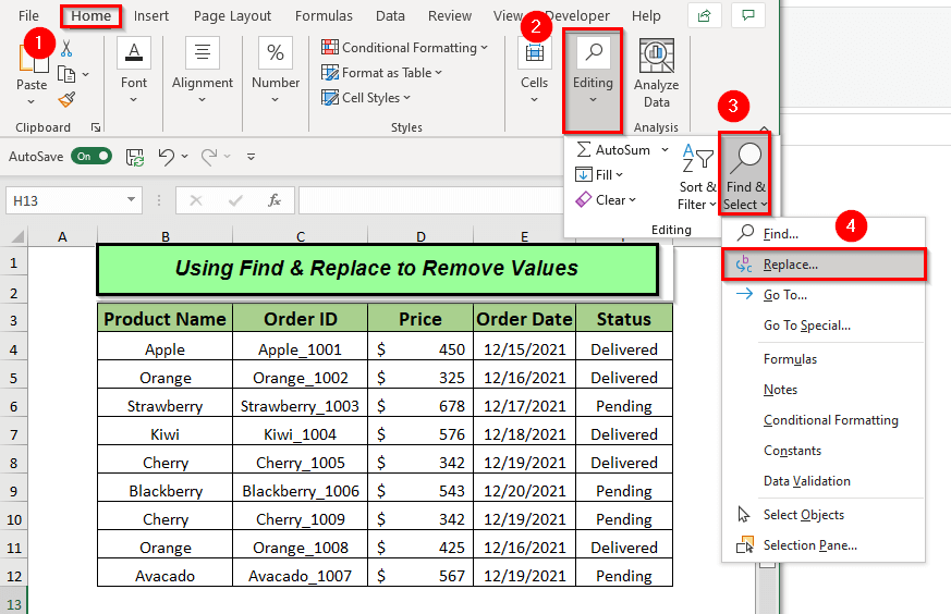
- A dialog box of Find and Replace will appear.
- In Find what, provide the value you want to find to remove it. I provided the value Delivered.
- Click Find All.
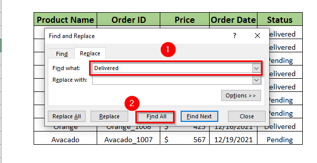
Here, you will see the cells that contain the Delivered value.
- Click Replace All.
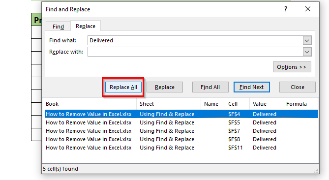
- A message about how many replacements occurred will appear. It has 5 replacements.
- Click OK.
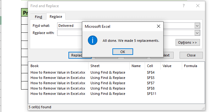
You will see the value you selected is removed.
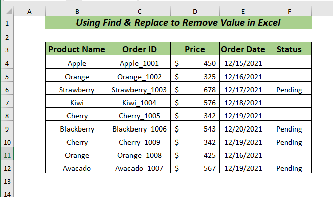
Method 5- Using Go To Special
Steps:
- Open the Home tab >> go to Editing group >> from Find & Select >> select Go To Special
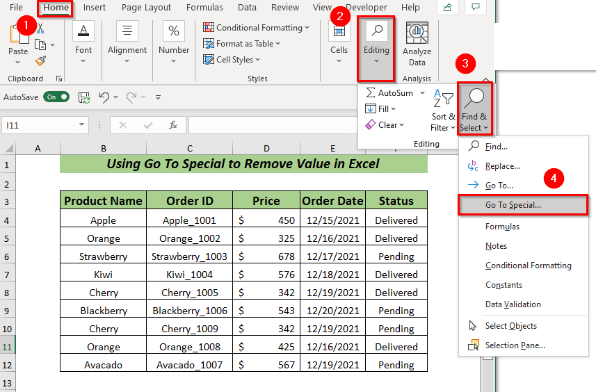
- A dialog box of Go To Special will pop up.
- From there select the type of your choice to remove. I selected Constants and Numbers.
- Click OK.
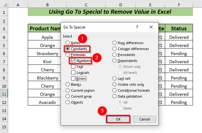
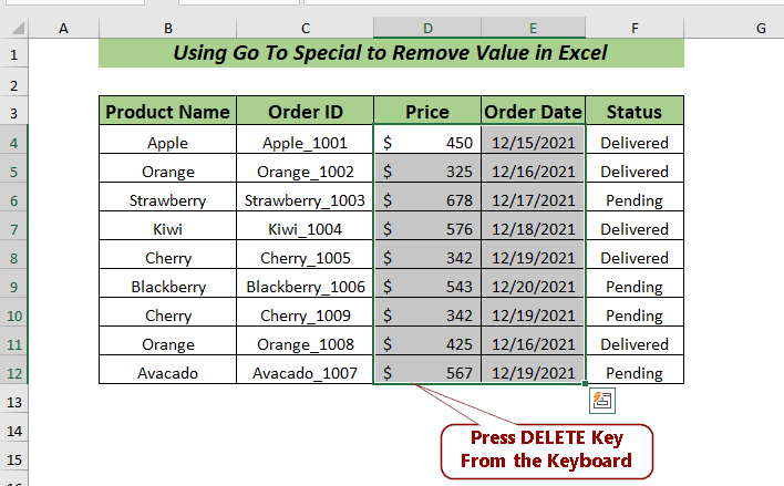
All the Constants Numbers values are selected.
- Press the DELETE key to remove the values.
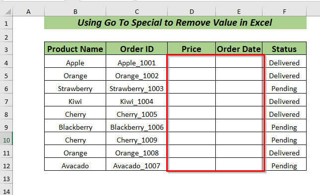
All the selected values are removed.
Method 6 – Using a Filter to Remove Value
Steps:
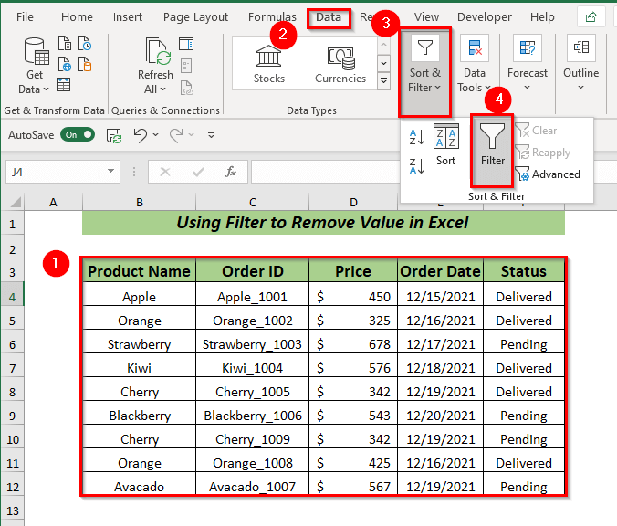
- Open the Data tab >> From Sort & Filter >> Select Filter
- The Filter will be applied here.
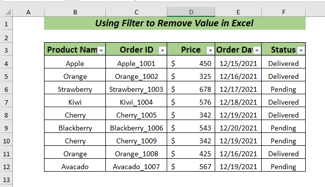
- Select any column to use the Filter options.
- Right-click.
- Unselect all, then select the value of your choice. I selected the Delivered value to apply Filters.
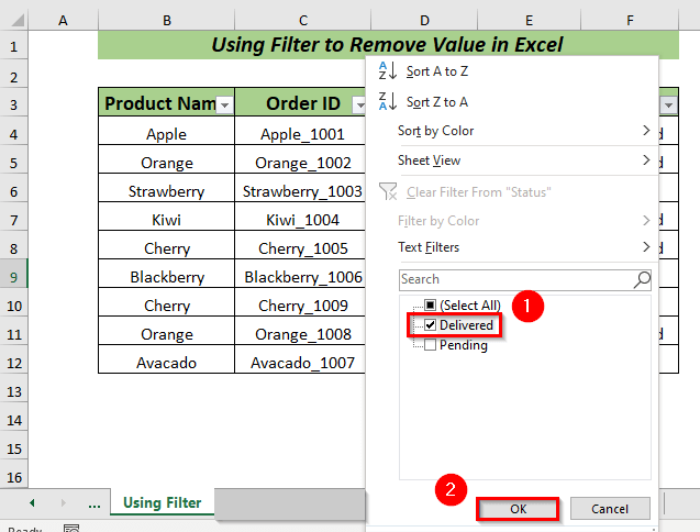 All the values that contain Delivered will be Filtered.
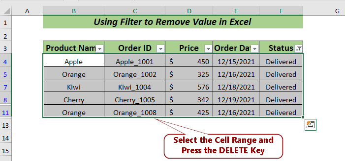
- Select the cell range and press DELETE.
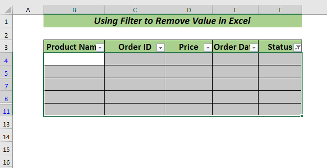
- All selected values are removed.
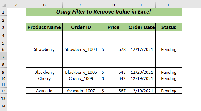
- Remove the Filter, and you will see all the values that contain the Delivered value are removed.
Method 7 – Using Text to Columns
Steps:
- Open the Data tab >> Select Text to Columns
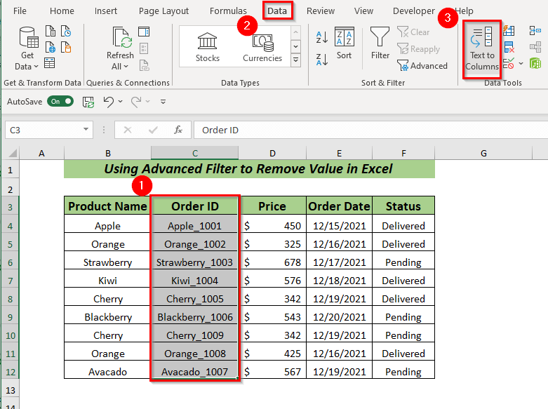
- A dialog box will pop up.
- From there, choose the data type I choose Delimited.
- Click Next
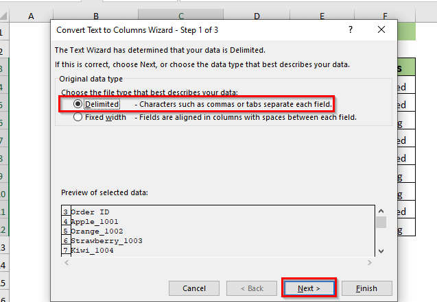
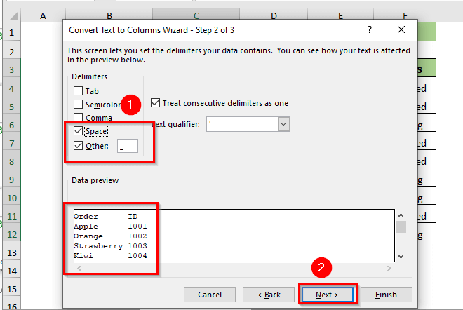
- Another dialog box will pop up.
- Select the Delimiters of your data. I selected Space (for the column header) and in Other given “_” as my data has underscore.
- Click Next.
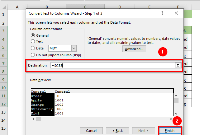
- A dialog box will pop up.
- From there, select the destination of your choice to place the separated values. I selected cell G3.
- Click Finish.
You will see the values of the Order ID column are separated into two columns.
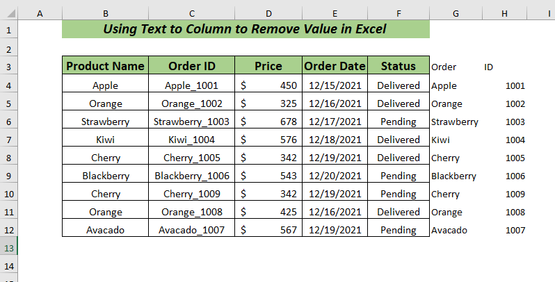
As I only need the Order ID number, I will cut the values of the ID column.
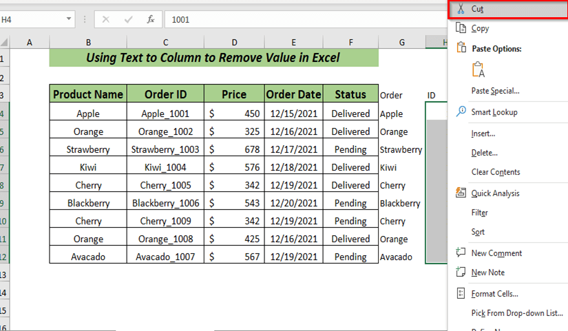
- Paste it into the Order ID column.
- Select the remaining Order column to remove.
- Press DELETE.
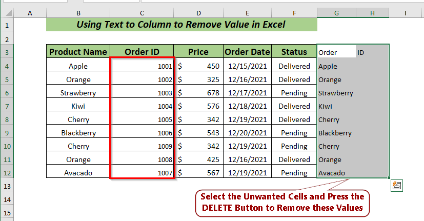
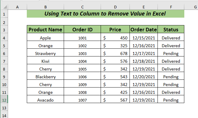
All the unwanted values are removed from the sheet.
Method 8 – Using Sort and Hide to Remove Value
Steps:
- Select the cell range to apply Sort. I selected the cell range B4:F12
- Open the Data tab >> Select Sort
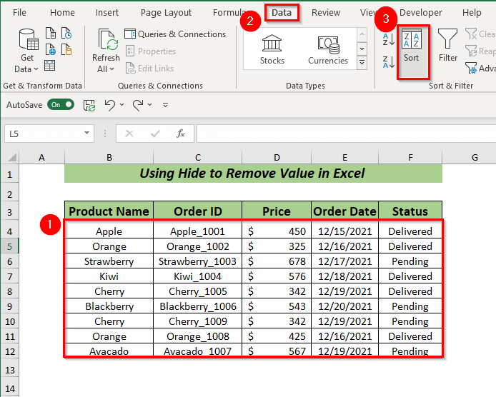 A dialog box will pop up. In Sort by I selected Status.
- Click OK.
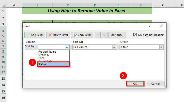
Here, Sort is applied, and all the values are sorted in A to Z Order according to the Status column value.
To hide the unwanted values, select the rows that contain unwanted values and then keep the cursor in the selected row number.
- Right-click.
- From the context menu, select Hide.
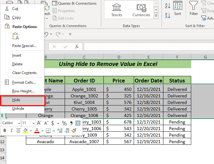
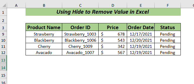
Unwanted values will be Hidden and removed.
Method 9 – Using VBA to Remove Value
Steps:
- Open the Developer tab >> Select Visual Basic (Keyboard Shortcut ALT + F11 )
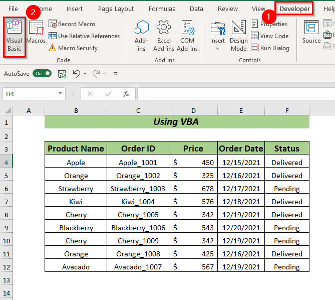
- It will open a new window of Microsoft Visual Basic for Applications.
- From there, open Insert >> Select Module
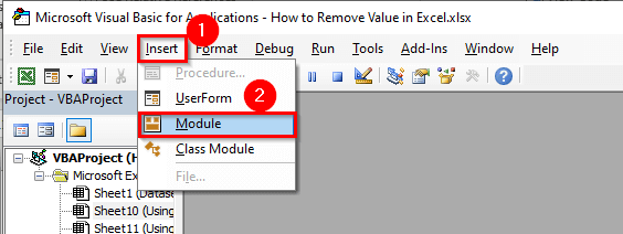
- A Module will open.
- Enter the following code in the opened Module:
Sub Remove_Values()
Range("B4:F7").Select
Selection.ClearContents
End Sub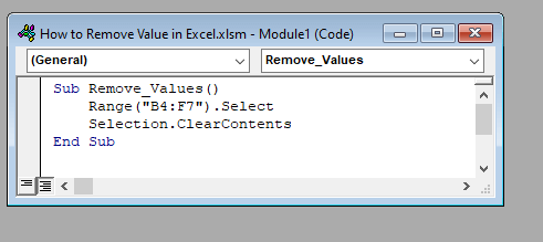
Here, I declared the Sub procedure Remove_Values
I used the Select method to select the given range B4:F7 (you can use the range of your choice or need)
Then, used the ClearContents method to remove the values from the given range.
- Save the code and go back to the worksheet.
- Open the View tab >> from Macros >> Select View Macros
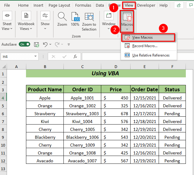
- A dialog box will pop up.
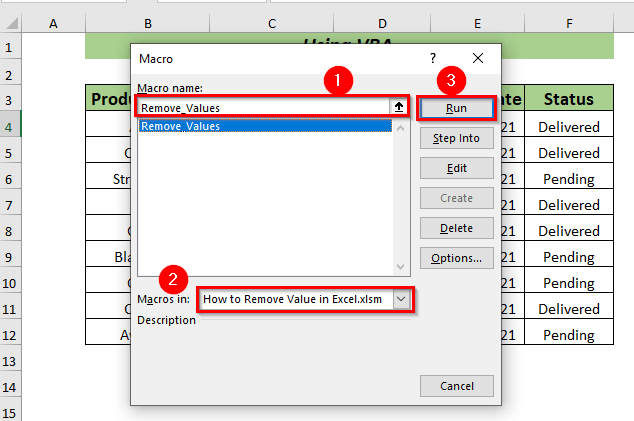
- From the Macro name, select the Remove_Values and the workbook within Macros in.
- Run the selected Macro.
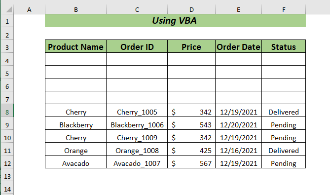
You will see the selected range values are removed.
Practice Section
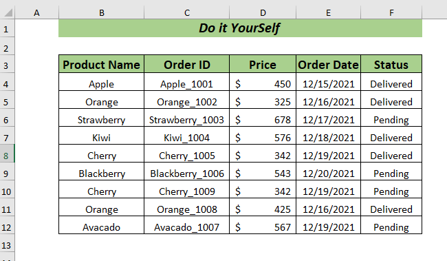
Below is a sheet to practice.
Download the Practice Workbook
Related Articles
- How to Remove Compatibility Mode in Excel
- How to Remove Drop Down Arrow in Excel
- How to Remove HTML Tags from Text in Excel
- How to Remove 0 from Excel
<< Go Back To Data Cleaning in Excel | Learn Excel
Get FREE Advanced Excel Exercises with Solutions!

