Dynamic Arrays Without VBA: FILTER, SORT, UNIQUE, and SEQUENCE Functions

Dynamic arrays in Excel return multiple results from a formula directly into a range of cells, eliminating the need for complex VBA code or manual processes. Excel’s most powerful dynamic array functions are FILTER, SORT, UNIQUE, and SEQUENCE. They simplify the data manipulation tasks. These functions automatically spill over adjacent cells, allowing you to create dynamic ranges that update instantly as your data changes. This tutorial will show how to use each function with practical examples.

Let’s consider a sales dataset to see the practical examples of dynamic arrays in Excel. We will use the FILTER, SORT, UNIQUE, and SEQUENCE functions to show how dynamic arrays work without VBA.

Using FILTER Function

The FILTER function returns an array based on certain conditions. This function can be used to extract specific data from a larger dataset.

Syntax:

=FILTER(array, include, [if_empty])

• array: The range of cells to filter data.
• include: Condition or logical test determining which rows to include in the output.
• [if_empty], [Optional]: If conditions are not fulfilled return any comment or blank space.

If you want to filter the Sales of the East region, you can insert the following formula in your selected cell.

Formula:

=FILTER(A2:G17, C2:C17=”East”, “No Data Found”)

This formula will filter out only the rows where the region is east. It will automatically extract sales data for the east region and spill over to adjacent cells.

Output:

Using SORT Function

The SORT function allows you to arrange data in ascending or descending order, based on one or more columns. It sorts the contents of a range or array.

Syntax:

=SORT(array, [sort_index], [sort_order], [by_col])

• array: It’s the range of cells to sort.
• [sort_index], [Optional]: The column or row index to sort by (default is 1).
• [sort_order], [Optional]: You can use 1 for ascending (default) and -1 for descending.
• [by_col], [Optional]: It sorts by columns (TRUE) or rows (FALSE, default).

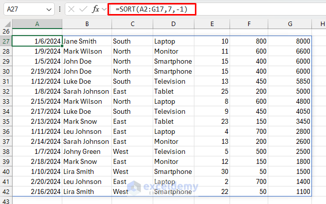
You can use the SORT function to sort sales by the highest sales values. Insert the following formula into your selected cell.

=SORT(A2:G17,7,-1)

This formula sorts the selected rows based on the sales column and returns the highest to lowest sales values.

• A2:G17: The range of cells.
• 7: The column index of the Sales column is 7.
• -1: Sort the rows in descending order.

Output:

Using UNIQUE Function

The UNIQUE function returns a list of distinct values from a dataset. It’s helpful to eliminate duplicates and get unique entries.

Syntax:

=UNIQUE(array, [by_col], [exactly_once])

• array: The range of cells to find unique values.
• [by_col], [Optional]: It checks uniqueness by row (FALSE, default) or by column (TRUE).
• [exactly_once], [Optional]: Return values that appear exactly once when set to TRUE.

If you want to know the product list from the sales data, you can use the UNIQUE function. Insert the following formula in your selected cell.

Formula:

=UNIQUE(D2:D17)

This formula returns the unique list of all products.

Output:

Using SEQUENCE Function

The SEQUENCE function generates a list of sequential numbers. You can use this function to create a serial list or an ordered list.

Syntax:

=SEQUENCE(rows, [columns], [start], [step])

• rows: Number of rows for the sequence.
• [columns], [Optional]: Number of columns for the sequence (default is 1).
• [start], [Optional]: Starting number (default is 1).
• [step], [Optional]: The step size between each number (default is 1).

If you want to generate a sequence of numbers from 1 to 10, you can insert the following formula in your desired cell.

=SEQUENCE(16)

This will return serial numbers from 1 to 16, each in a separate row in the sales data.

Output:

To generate a sequence from 5 to 60 and increase each number by 5 you can use the following formula.

=SEQUENCE(4, 3, 5, 5)

Explanation:

• 4: The output will contain 4 rows.
• 3: This will show the output in 3 columns.
• 5: This is the number where the sequence starts (the first value will be 5).
• 5: It’s the increment between each value (each number increases by 5).

Output:

Combining Dynamic Array Functions

You can combine all these functions for more powerful results. You can filter sales values from the north region and sort the filtered values from lowest to highest sales by combining the UNIQUE, SORT, and FILTER functions.

Formula:

=UNIQUE(SORT(FILTER(A2:G17, C2:C17=”North”), 1, 1))

This will filter unique rows from A2:G17 where the region is north then it will sort the rows based on the sales column from lowest to highest.

Output:

Conclusion

By using FILTER, SORT, UNIQUE, and SEQUENCE functions in Excel you can streamline dynamic arrays without the need for VBA. These dynamic array functions automatically adjust the result size to match the data and automatically update datasets that respond to your data changes. These functions are incredibly useful for anyone working with large datasets and wanting to avoid manual recalculations or complex formulas.