Data cleaning is crucial for performing data analysis and calculations and it is the first step in data preparation and formatting. Data cleaning means removing inconsistencies, errors, and unwanted formatting. Both Microsoft Excel’s Power Query and Google Sheets’ REGEX functions are powerful for advanced cleaning. Let us show you how to use Power Query and Google Sheets’ REGEX functions for advanced data cleaning while comparing them.
Excel’s Power Query
Power Query is a built-in Excel feature that provides a user-friendly interface for data transformation and data cleaning. It cleans and formats data without any complex formulas. Power Query imports data from various sources and offers robust data connectivity. It has flexible features to perform complex data-cleaning tasks.
Google Sheets’ REGEX functions
Google Sheets’ REGEX functions use regular expressions to find patterns within text data, making it ideal for parsing, formatting, or validating text entries.
- REGEXREPLACE: Replaces text matching a regular expression with specified text.
- =REGEXREPLACE(text, regular_expression, replacement)
- REGEXMATCH: Checks if a text string matches a specified regular expression.
- =REGEXMATCH(text, regular_expression)
- REGEXEXTRACT: Extracts matching substrings from text based on a regular expression.
- =REGEXEXTRACT(text, regular_expression)
These functions are useful for data cleaning, pattern recognition, and dynamic text manipulation.
Let’s consider a raw dataset containing wrong formatting, unwanted characters, errors, blank spaces, and so on. By using Excel’s Power Query and Google Sheets’ REGEX functions we will show you the advanced data cleaning while comparing each other.
Removing Unwanted Characters
Clean a dataset of phone numbers containing unwanted characters like parentheses, dashes, or spaces.
Power Query
- Select the data range.
- Go to the Data tab >> select From Table/Range.
- Power Query editor will pop up. Select the column. We selected the Phone Number column.
- Go to the Transform tab >> select Replace Values.
- Replace Values dialog box will pop up;
- In the Value to Find box: Enter unwanted characters ((, ), -, ) individually.
- In the Replace with box: Keep it empty or if you have a value to replace with you can insert that value.
- Click OK.

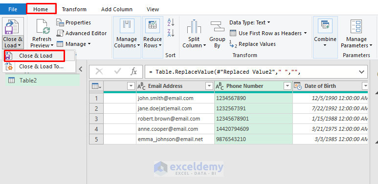
- Select Close & Load to bring the cleaned data back to Excel.

Google Sheets’ REGEXREPLACE Function
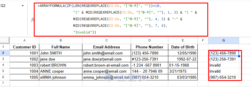
Let’s clean data along with formatting in Google Sheets by using the REGREPLACE function. Insert the following formula in cell G2.
=ARRAYFORMULA(IF(LEN(REGEXREPLACE(D2:D6, "[^0-9]", ""))=10,
                 "(" & MID(REGEXREPLACE(D2:D6, "[^0-9]", ""), 1, 3) & ") " &
                 MID(REGEXREPLACE(D2:D6, "[^0-9]", ""), 4, 3) & "-" &
                 MID(REGEXREPLACE(D2:D6, "[^0-9]", ""), 7, 4),
                 "Invalid"))
This formula will remove all non-numeric characters. Then, it will check if the cleaned number has exactly 10 digits. If it’s valid, format it as (XXX) XXX-XXXX; otherwise, it returns “Invalid”.

Google Sheets’ REGREPLACE Function
You can use the following formula to clean unnecessary special characters.
Formula:
=REGEXREPLACE(D2, "[^a-zA-Z0-9]", "")
This [^a-zA-Z0-9] pattern removes any character that isn’t a letter or digit.
If you are familiar with regular expressions, you can use the REGREPLACE function, it removes any characters except letters or digits within a single formula.

Standardizing Text Case
The dataset may contain mixed text; you can convert all text entries to lowercase or title case.
Power Query
Open Power Query by selecting the data range and navigating to the Data tab >> select From Table/Range.
- Select the column with text to transform.
- Go to the Transform tab >> select Capitalize Each Word.

Google Sheets PROPER Function
In Google Sheets’ there isn’t a way to capitalize each word purely with regex, as Google Sheets’ REGEXREPLACE doesn’t support UPPER and LOWER functions directly within regex patterns or replacements. You can use external functions like PROPER, UPPER, or LOWER.
=PROPER(B2)
This formula ensures each word is capitalized, and any non-first letters are converted to lowercase.

Splitting Data by Delimiter
You can split any merged texts or names into separate columns by delimiter. Let’s clean the data by using Power Query and Google Sheets’ REGEX functions.
Power Query
Open Power Query by selecting the data range and navigating to the Data tab >> select From Table/Range.
- Choose the column containing names.
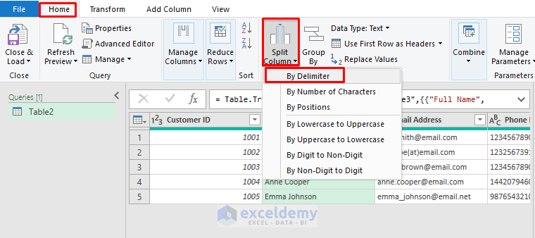
- Go to Home tab >> from Split Column > select By Delimiter.

- In Split Column by Delimiter dialog box;
- In Select and enter delimiter: choose a Space( ).
- Click OK.

- Rename the resulting columns to “First Name” and “Last Name”.

Google Sheets REGEXEXTRACT Function
You can use the REGEXEXTRACT function to split data by delimiter. Insert the following formula in your selected cell.
=REGEXEXTRACT(E9, "^([^ ]+) (.+)$")
This formula separates the last name and first name into two cells. It uses additional columns as needed.

When to Use Power Query vs. Google Sheets REGEX
Power Query is the most useful for basic to advanced data cleaning. It is ideal for more extensive, structured data transformation with a user-friendly interface. It’s efficient when working with complex datasets, structured joins, and merging data.
Google Sheets REGEX functions are perfect for quick text-based operations and specific text extraction within individual cells. REGEX functions are especially helpful if you’re comfortable with regular expression syntax.
Conclusion
Power Query and Google Sheets’ REGEX functions provide complementary tools for data cleaning. Power Query is ideal for Excel users needing batch transformations on large datasets, while Google Sheets REGEX functions offer flexibility for text-based operations in smaller datasets. You can use both effectively for powerful, streamlined data cleaning! By understanding both tools, you can handle most cleaning tasks whether you’re in Excel or Google Sheets!
Get FREE Advanced Excel Exercises with Solutions!

