When to Use Array Formulas vs. Dynamic Arrays in Excel

Array formulas and dynamic arrays are powerful tools for complex batch calculations by managing multiple values simultaneously. Both are used to manipulate data across multiple cells, but they have key differences that influence when and how to use each effectively. Array formulas are used in the older Excel versions whereas dynamic arrays are available in newer Excel versions. This article will show practical examples to help you understand when to use array formulas versus dynamic arrays in Excel.

What are Array Formulas?

Array formulas are traditional formulas also known as legacy formulas that can return multiple values to a single cell or a range of cells. They are typically entered by pressing Ctrl + Shift + Enter. If you’re using a version of Excel before 2019 and MS Office 365, array formulas are your only option for working with arrays. To sum or average specific values based on conditions across multiple rows or columns, array formulas are invaluable. Array formulas allow you to define constants within formulas, such as {1, 2, 3}, and use them across calculations.

What are Dynamic Arrays?

Dynamic arrays, introduced in Excel 2019 and MS Office 365, simplify working with arrays by allowing formulas to spill results across multiple cells without pressing Ctrl + Shift + Enter. Dynamic arrays automatically resize when source data changes, which makes them more versatile for modern use cases. Dynamic arrays simplify calculations by spilling results into adjacent cells automatically. Dynamic arrays introduced functions like UNIQUE, SORT, FILTER, SEQUENCE, etc, which allows us to easily work with ranges, sort data, filter lists, or create sequences. Dynamic arrays update and resize as data changes, making them more responsive to live data and updates.

Let’s consider a sample dataset to explore some practical examples by using array formulas and dynamic arrays.

Extracting Unique Values

Let’s extract unique values from the product list by using both array formulas and dynamic arrays.

Array Formulas

To extract a unique product list by using array formulas you will need to use the combination of IFERROR, INDEX, MATCH, and COUNTIF functions.

• Insert the following formula in cell H2.
• Press Ctrl + Shift + Enter to make it an array formula (you’ll see curly braces {} around the formula in the formula bar).
• Drag the formula down until you see blanks, indicating that all unique products have been extracted.

Formula:

=IFERROR(INDEX($C$2:$C$14, MATCH(0, COUNTIF($H$1:H1, $C$2:$C$14), 0)), "")

This array formula works by using COUNTIF to check if each product has already been listed in the cells above. When MATCH finds a product not yet listed, INDEX retrieves it from column C. IFERROR handles any errors when there are no more unique products to extract.

Output:

Dynamic Arrays

Let’s perform a similar task by using only the UNIQUE function. Insert the following formula in cell I2 and press Enter.

Formula:

=UNIQUE(C2:C14)

The UNIQUE function will spill all the unique values into adjacent cells automatically. Dynamic arrays make this task much simpler, and they automatically adjust when data in C2:C14 changes.

Output:

Sum Based on Condition

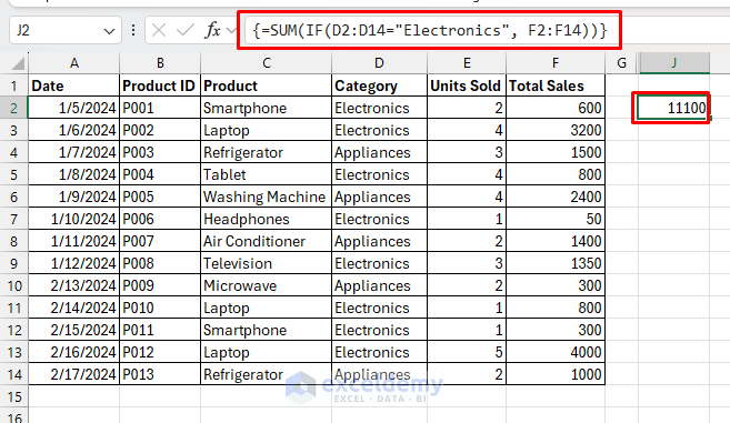
Suppose you have sales data in F2:F14 with the corresponding category in D2:D14. You want to sum sales where the category is “Electronics”.

• Insert the following formula in cell J2.
• Press Ctrl + Shift + Enter to turn it into an array formula.

Array Formulas

Formula:

=SUM(IF(D2:D14="Electronics", F2:F14))

The IF function extracts the sales value based on the category, and the SUM function sums the Total Sales.

Output:

Dynamic Arrays

To calculate the total sales based on category using the SUMIFS dynamic array function. Type the formula in cell K2 and press Enter.

Formula:

=SUMIFS(F2:F14, D2:D14, "Electronics")

The SUMIFS dynamic array function calculates the total sales based on the condition. It allows a simpler solution without needing Ctrl + Shift + Enter and it updates dynamically.

Output:

Filtering Data Based on Criteria

Imagine you want to filter sales data where the Total Sales is greater than $1000.

Array Formulas

You can use the combination of INDEX, SMALL, IF, and ROW functions to create an array formula to extract total sales greater than $1000.

• Enter the formula in cell L2.
• Press Ctrl + Shift + Enter.
• Drag the formula down to get all the sales values over $1000.

Formula:

=IFERROR(INDEX($F$2:$F$14, SMALL(IF($F$2:$F$14>1000, ROW($F$2:$F$14)-ROW($F$2)+1), ROW(1:1))), "")

This formula extracts values from the range $F$2:$F$14 that are greater than 1000. The IF condition identifies rows where values exceed 1000, and SMALL retrieves the smallest eligible row number each time the formula is dragged down, providing the next qualifying value. IFERROR ensures that once no more values meet the condition, the formula returns a blank instead of an error.

Output:

Dynamic Arrays

You can use the FILTER function to get total sales greater than $1000. Enter the formula in cell M2 and press Enter.

Formula:

=FILTER(F2:F14, F2:F14>1000)

This formula will spill sales over $1000 into the cells below automatically. With dynamic arrays, you get a cleaner, auto-spilling formula that updates based on changes in F2:F14.

Output:

Generating a Sequence Number

Suppose you want to create a sequence of numbers to order the sales data.

Array Formulas

You can use the ROW and INDIRECT functions to create array formulas for generating sequences.

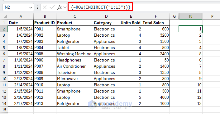
• Enter the formula in N2.
• Press Ctrl + Shift + Enter.
• This will populate numbers 1 to 13 in the selected range.

Formula:

=ROW(INDIRECT("1:13"))

The formula generates an array of row numbers from 1 to 13. The INDIRECT (“1:13”) creates a reference to rows 1 through 13. ROW(…) then returns the row numbers for this range, resulting in {1; 2; 3; …; 13}.

Output:

Dynamic Arrays

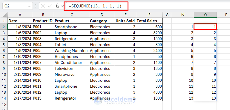
By using the dynamic SEQUENCE array function, you can easily create any type of sequence. Insert the formula in cell O2 and press Enter.

Formula:

=SEQUENCE(13, 1, 1, 1)

The dynamic SEQUENCE function is simpler, spilling results automatically across cells, and can be customized to start and increment at different values. It will create sequence numbers from 1 to 13 within a single click.

Output:

Choosing Between Array Formulas and Dynamic Arrays

Use Array Formulas If:

• You’re working on an older Excel version.
• You’re performing legacy calculations that don’t require spilling or batch calculations

Use Dynamic Arrays If:

• You have access to Excel 2019, MS Office 365 or later.
• You want automatic updates and spill ranges, making your formulas flexible and dynamic.
• You are looking for simplified ways to work with large datasets.

Conclusion

The choice of using array formulas or dynamic arrays mostly depends on your Excel version and specific needs. Dynamic arrays bring ease of use, versatility, and automatic updates while traditional array formulas maintain compatibility with older versions. These examples highlight how dynamic arrays simplify complex tasks, making your Excel worksheets more efficient and responsive. By understanding the differences, you can leverage the power of both types of array formulas to handle complex calculations more effectively.