How to Use Cell References in Excel Formula (All Possible Ways)

The use of cell references in an Excel formula is very important when formulas are copied and pasted to other cells. Excel worksheet is made of cells and we refer to these cells by specifying row number and column number. We can use these cell references of the same worksheet or from a different worksheet while creating formulas. Basically, there are three types of cell references we can use in excel,

Relative Cell Reference
Absolute Cell Reference
Mixed Cell Reference

Uses of Different Cell References in Excel Formula

Here we’ll work on a dataset of a list of fruit items in a super shop in Australia. The dataset has a price column that shows the product of Unit Price and Quantity of the fruit items. We’ll first find out the Price as a product of Unit Price and Quantity and show the use of relative cell reference. One fixed tax rate will be used to demonstrate the use of fixed cell reference and variable tax rate to demonstrate the mixed cell reference.

1. Use of Relative Cell Reference in Formula in Excel

What is Relative Cell Reference in Excel?

In Excel, all cell references are relative, by default. Relative cell reference changes according to the relative position of rows and columns while copied and then pasted through a range of cells. In the following example, we’ll see how the formula D5*E5 changes like D6*E6, D7*D7, and D9*E9 at last.

How to Use Relative Cell References in Formula in Excel

In this example, we’ll copy and paste the formula which calculates the product of Unit Price and Quantity through the other column cells to show the use of relative cell reference. Let’s follow the example:

Steps:

In cell F5, write the following formula to calculate the Price as a product of the Unit Price and Quantity

=D5*E5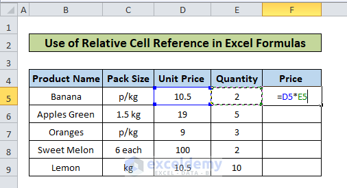

Then hit Enter and the result is 21 (=10.5*2).
Now pick the fill handler for cell F5 at the bottom right corner of the cell, hold and drag it down to the cells F6:F9 of column F.

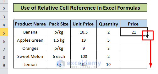
The above steps copied the formula of cell F5 and then pasted it to F6:F9 with relative references.

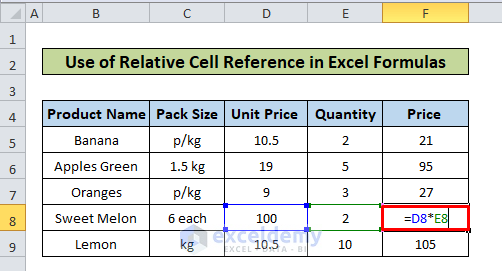
Now to check, click on any of the cells from F6:F9. Here we clicked on cell F8 which shows the formula as a product of cells D8 and E8, relative to the row number of cell F8.

2. Absolute Cell Reference in Excel Formula

What is Absolute Cell Reference in Excel?

In different calculations, we use a constant value in the formula that doesn’t change relatively with the rows and columns positions. That’s how we can use an absolute cell reference in such a formula. In the following illustration, we’ll see how to get different Price After Tax values while keeping the tax rate value constant using absolute cell reference $C$11.

How to Use Absolute Cell References in Excel Formula

In this example, we calculated the Price After Tax value on a fixed tax rate of 7.5%, stored in cell C11. To get this we used the Total Price values that were calculated in the previous example. Let’s dive into the example:

Steps:

To calculate the Price After Tax, write the following formula in cell G5–

=F5+(F5*$C$11)

To make cell C11 an absolute reference we put the $ sign before the column value C and also before the row value 11, which is $C$11. Here F5 is a relative reference that will change relative to the row number downwards.

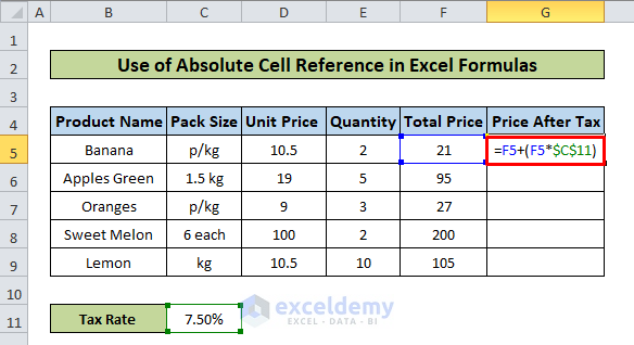
After this hit Enter and the result is 22.58 (=21+21*.075).
To copy and paste the formula to cells G6:G9 locate the fill handler, drag it down to the cells and finally, release the cursor.

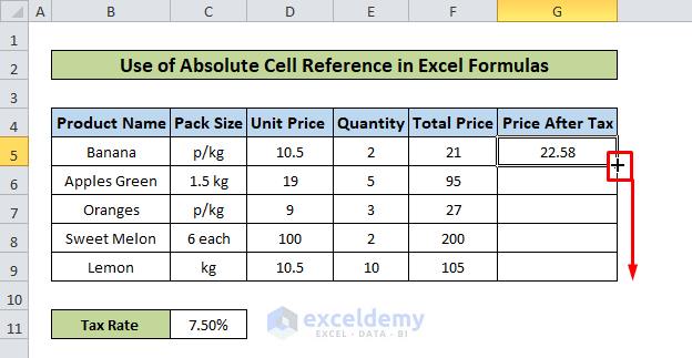
The above steps copied the formula of cell F5 and then pasted it to F6:F9 with absolute references.

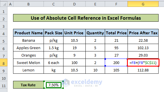
In the final result, we see each of the values of the Price After Tax column used the absolute cell reference $C$11. Let’s click on cell G8. It shows the formula which contains the relative cell reference F8 according to the row number of G8 but the absolute cell reference $C$11 remains constant.

Read More: How to Hard Code in Excel

3. Write Formula Using Mixed Cell Reference in Excel

What is Mixed Cell Reference in Excel?

The mixed cell reference is a combination of relative and absolute cell references together. In this case, we put one part of the cell reference relative and the other part absolute vice-versa.

How to Write a Formula Using Mixed Cell References in Excel

In this illustration, we want to calculate Price After Tax for three different Tax Rates that are located in cells C13, D13, and E13. When we are applying the formula for a product like Banana, we want three Price After Tax values for three different tax rates. That means tax rate cell reference has to be relative row-wise. Again for a specific duration like Jan-Apr, we should have a fixed tax rate to get the Price After Tax values which require absolute tax rate column-wise. Let’s follow the example below to get a clear understanding.

Steps:

In cell G6, write the following formula-

=$F6+($F6*C$13)

Here we put the tax rate cell reference as C$13 which is mixed. We put the $ sign before the column value 13 to make it absolute column-wise and left the row value C without the $ sign as it’ll be relative row-wise.

There is another way to look at the formula. $F6 is also a mixed cell reference. It is relative through the column cells and absolute through the row cells while calculating the Price After Tax values.

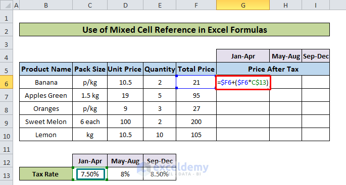
Let’s hit Enter and the output is 58 (=21+21*0.075).
Now locate the fill handler and drag it to the right to calculate values for different tax rates of different time durations.

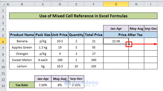
The output shows three Price After Tax values for three different tax values.

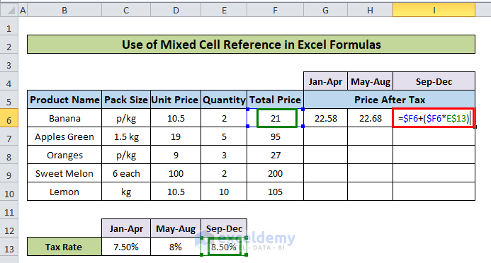
To check double click on cell I6. In the formula, we can see the tax rate cell reference is E$13 (C$13 in cell G6 formula) which is relative row-wise. On the other hand, the total price cell reference $F6 didn’t change as it was in the formula for G6 which is absolute row-wise.

This time locate the fill handler at the right bottom corner of cell G6 and drag it down to G6:G10.

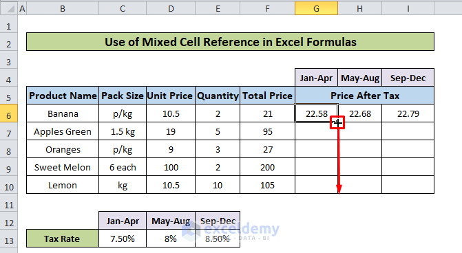
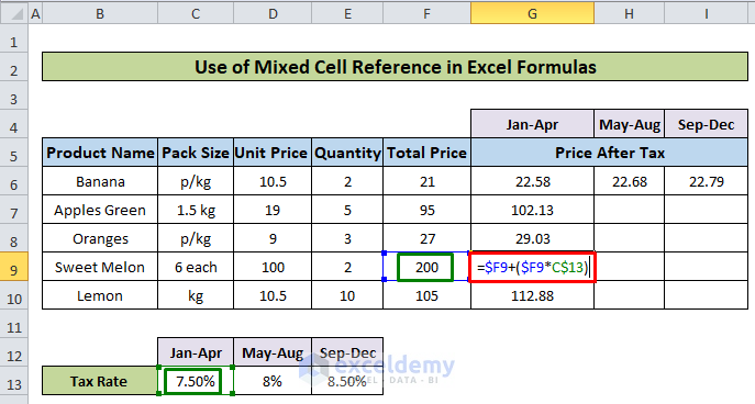
From the results, let’s double click cell G9 to explain what happens here. In the formula, we can see the tax rate cell reference is C$13 (also C$13 in cell G6 formula) which is absolute column-wise. On the other hand, the total price cell reference $F6 did change to $F9 which is relative column-wise.

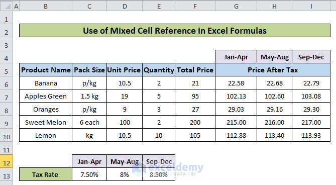
Finally, we get all the values for Price After Tax following the previous steps.

Notes

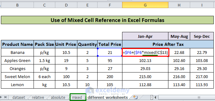
We can also use a cell reference from one worksheet in a formula that is in another worksheet i.e. across multiple worksheets. In the following illustration, we used the mixed tax rate cell reference from the mixed worksheet. Although the formula is in the worksheet which is named as ‘different worksheet’. For this, we need to put the worksheet name in a quote and an exclamation (!) sign after that. And then put the cell reference. See the example below:

Download Practice Workbook

Download this practice workbook to exercise while you are reading this article.

Cell References.xlsx

Conclusion

Now, we know how to use different types of cell references in Excel. Hopefully, it would encourage you to use this functionality more confidently. Any questions or suggestions don’t forget to put them in the comment box below.

<< Go Back to Cell Reference in Excel | Excel Formulas | Learn Excel

Get FREE Advanced Excel Exercises with Solutions!