How to Use COUNTIF with SUBTOTAL in Excel (2 Methods)

In this article, we’ll demonstrate how to count filtered data using the COUNTIF function together with the SUBTOTAL function.

Download the Practice Workbook

SUBTOTAL COUNTIF.xlsx

2 Methods for Using COUNTIF with SUBTOTAL in Excel

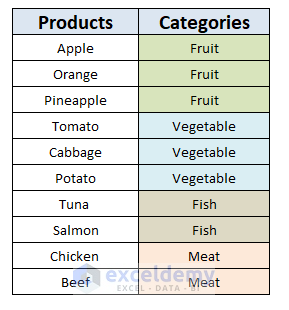
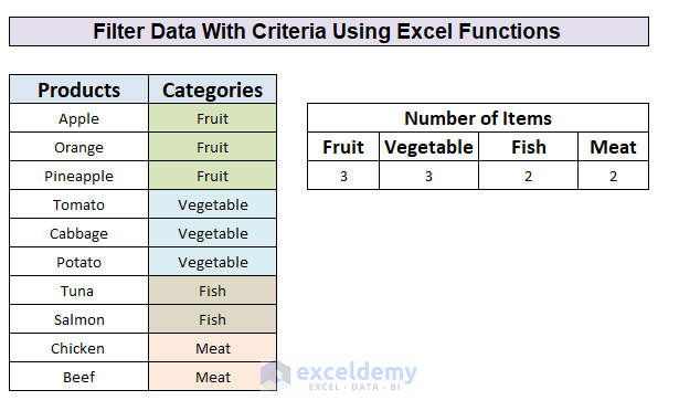
We’ll use the following dataset, which contains a list of products in 4 different categories, to find the number of visible rows only. We’ll find out the number of products under each category.

Method 1 – Counting Filtered Data With Criteria Using Excel Functions

Usually, the SUBTOTAL function cannot handle criteria that are given by the COUNTIF function. But we can filter the count number using the SUMPRODUCT function with both the SUBTOTAL function (via the OFFSET function) and the criteria.

Steps:

In cell E6 enter the following formula:

=SUMPRODUCT((C5:C14=C5)*(SUBTOTAL(103,OFFSET(C5,ROW(C5:C14)-MIN(ROW(C5:C14)),0))))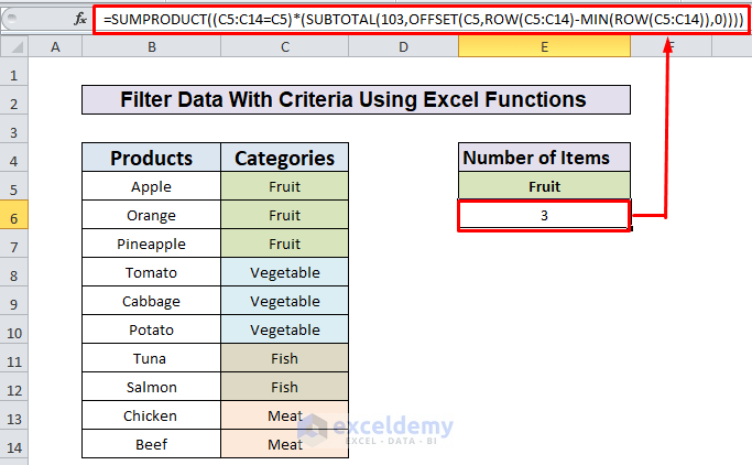

Formula Breakdown:

The SUMPRODUCT function takes arrays as its input. In this formula, we put the first input array as the criteria and the second input array handles the visibility.

The criteria are:

=(C5:C14=C5)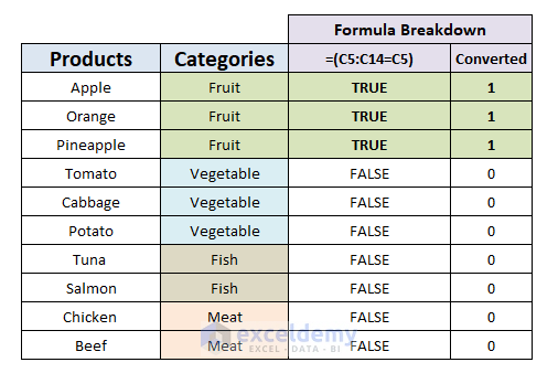

This checks the value of C5 (Fruit) against the range C5:C14. It outputs an array shown in the screenshot below. As this array is in the multiplication form in the formula, it resolves into an array of 1’s and 0’s.

{1, 1, 1, 0, 0, 0, 0, 0, 0, 0, 0}

In the second part of the formula, the SUBTOTAL function returns a single value as an output. But we need to put an array input in the SUMPRODUCT function, so we use the OFFSET function as an input of the SUBTOTAL function, one reference per row, which returns one result per row. This requires putting an array that contains one number per row starting with zero as the input of the OFFSET function.

Enter the formula below to acquire this array:

=ROW(C5:C15)-MIN(ROW(C5:C14))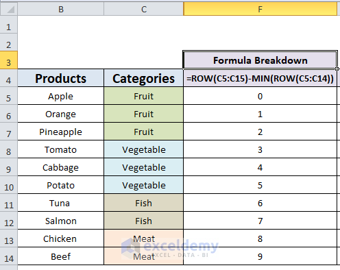

Put the above formula into the OFFSET function:

=OFFSET(C5,ROW(C5:C14)-MIN(ROW(C5:C14)),0)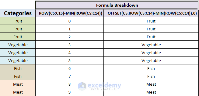

The SUBTOTAL function returns an array of 1’s and 0’s.

=(SUBTOTAL(103,OFFSET(C5,ROW(C5:C14)-MIN(ROW(C5:C14)),0)))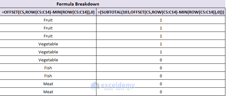

Now we can apply the formula:

=SUMPRODUCT( criteria * visibility )

Enter the following formula into any blank cell:

=SUMPRODUCT(D5:D14*H5:H14)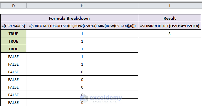

The range D5:D14 represents the criteria and the range H5:H14 represents visibility. The result is 3 which is the number of Fruit products in the Products list.

Similarly, we can filter and return the number of products for each category.

Similar Reading

Method 2 – Using COUNTIFS Function to Count Filter Data with Criteria by Adding a Helper Column

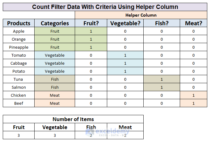
First we’ll add a helper column and then use the SUMIFS function to count the number of products based on their categories.

Steps:

In cell D4, enter the following formula:

=IF(C4="Fruit",1,0)

This formula checks if the value of cell C4 is Fruit or not. If the value is Fruit then it will show 1 else 0.

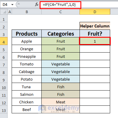
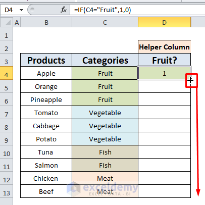
Using the Fill Handle, copy the formula to the rest of the column.

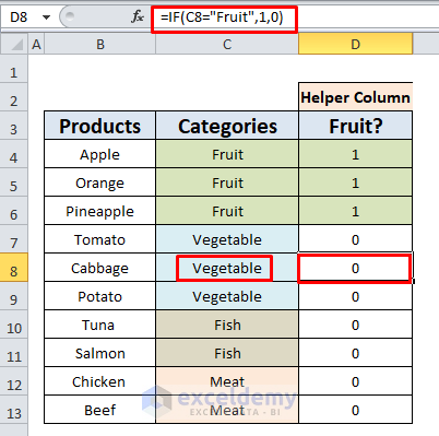
The result is that the cells with Fruit category show 1 and the cells with categories other than Fruit show 0 as output.

Enter the following formula in a blank cell (in this example cell I7) where you want to store the result.

=COUNTIFS(C4:C13,"Fruit",D4:D13,"1")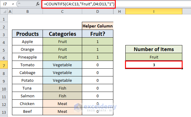

The COUNTIFS function checks two criteria in two ranges and returns the number of matches. In the range C4:C13 it matches for Fruit and in the range D4:D13 it matches for 1.

The number of products in each category is returned.

Notes

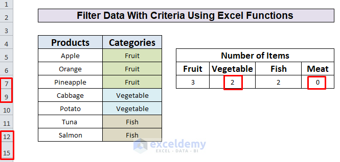
The SUBTOTAL function uses a function_num as an argument that controls the behavior of the function. Depending on the function_num value, the SUBTOTAL function can calculate AVERAGE, SUM, MAX, MIN, COUNT, etc. of a range of values. Here we used 103 which ignores the hidden rows while applying the COUNTA function.

For example, here we hide row 8, which reduces the number of products from the Vegetable category from 3 to 2. We also hide rows 13 and 14 which contain products of the Meat category, reducing the count to 0.