We have an Excel worksheet that contains information on various outlets of a chain restaurant all across the United States. The Excel worksheet contains sales and expenditures for the restaurants. We will use comparison operators i.e., greater than (>) and less than (<) to find out if an outlet earned profit or incurred loss. We will also use these greater than and less than Excel operators to count and sum all the sales amounts above or below a certain amount, determine the tax rate based on the sales amount, for conditional formatting, and apply them to text values.
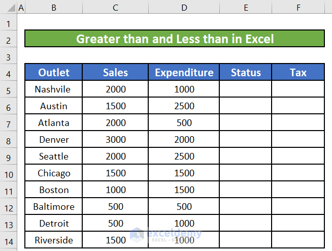
Method 1 – Greater Than and Less Than in Excel to Compare Cell Values
Steps:
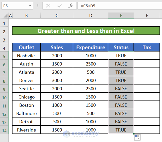
- Consider the formula in cell E5 below. We are comparing the sales amount in cell C5 with the expenditure amount in cell D5.
=C5>D5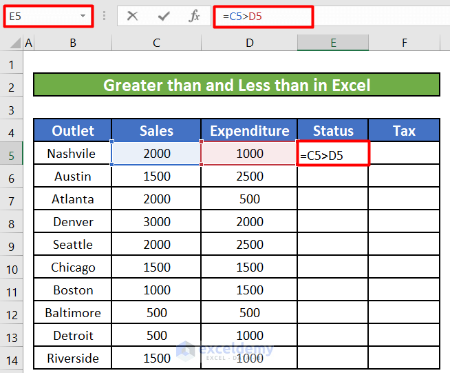
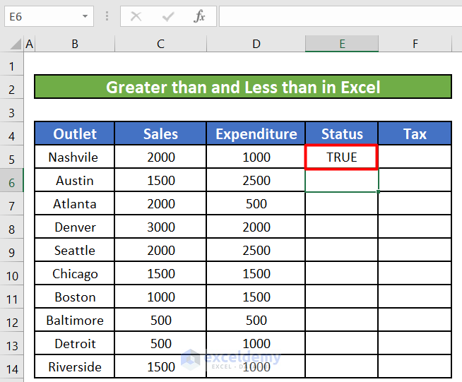
- We will get the Boolean value TRUE in cell E5. The sales amount (C5) is greater than the expenditure amount (D5). Hence, the cell is showing TRUE.
- We will do the same for the rest of the cells in this column by dragging down the fill handle.
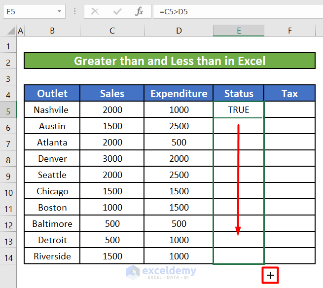
- All the cells in the Status column will show boolean values.
- We can also use both conditional operators together to compare if any two values are different with the following formula:
=C5<>D5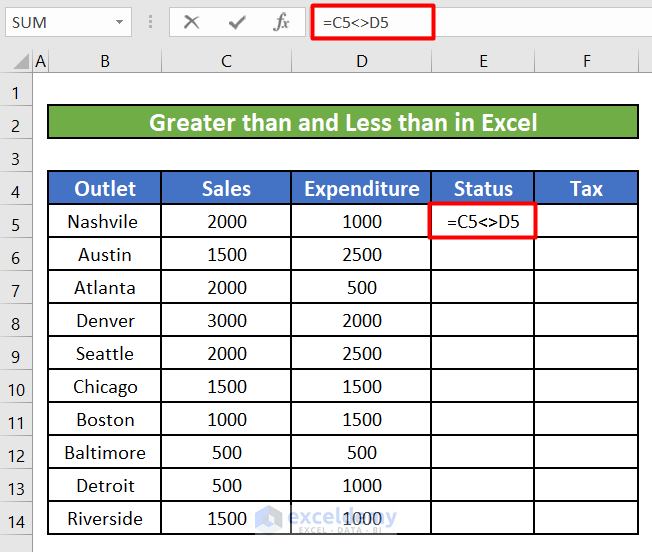
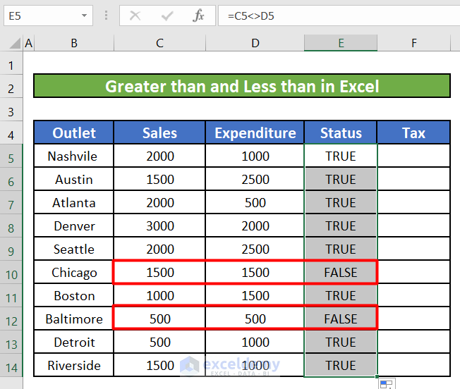
- As the Sales (C5) and Expenditure (D5) values are not equal, the formula will return TRUE. If we drag the fill handle to autofill the rest of the cells, it will return boolean values for every cell comparing the corresponding Sales and Expenditure values in the respective rows.
Read More: How to Use Greater Than or Equal to Operator in Excel Formula
Method 2 – Greater Than and Less Than Excel Comparison Operators in Arguments of Excel Functions
We’ll find out if an outlet is gaining profit or incurring a loss, then count and sum up all the sales amount above $1000.
Case 2.1 – Comparison Operators with the IF Function
Steps:
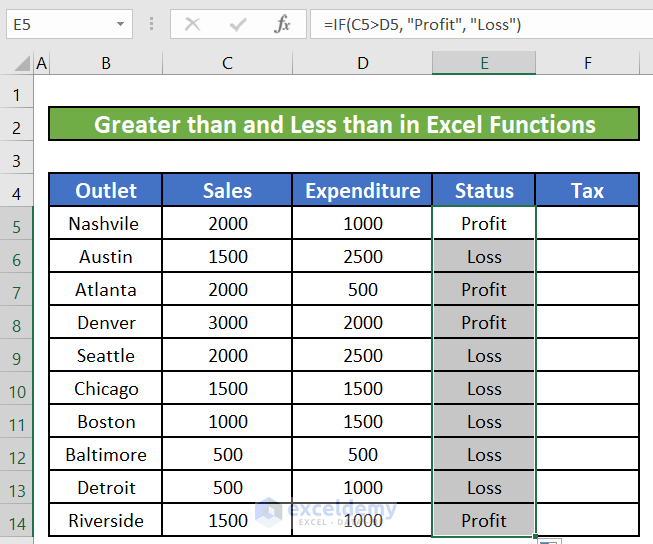
- Consider the following formula in cell E5,
=IF(C5>D5, "Profit", "Loss")
- The IF function will compare the Sales with Expenditure. If the Sales are greater than the Expenditure, then it will return the value “True”. If Sales are less than Expenditure, then it will return “Loss”.
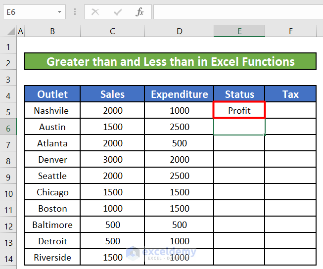
- We can drag the fill handle down to fill the other cells in this column with the same formula for the respective cells.
Case 2.2 – Comparison Operators with the COUNTIF Function
Steps:
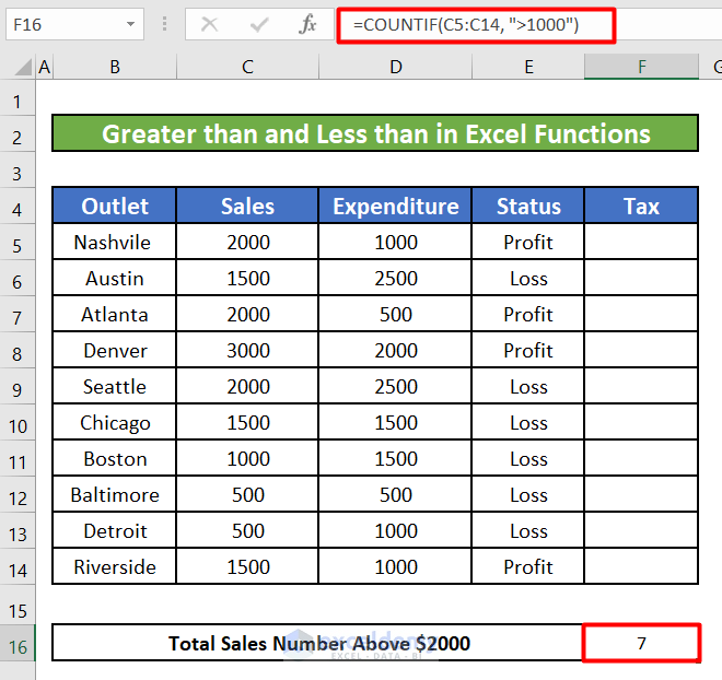
- To count all the sales amounts that are greater than $1,000, use the following formula in cell F16.
=COUNTIF(C5:C14, ">1000")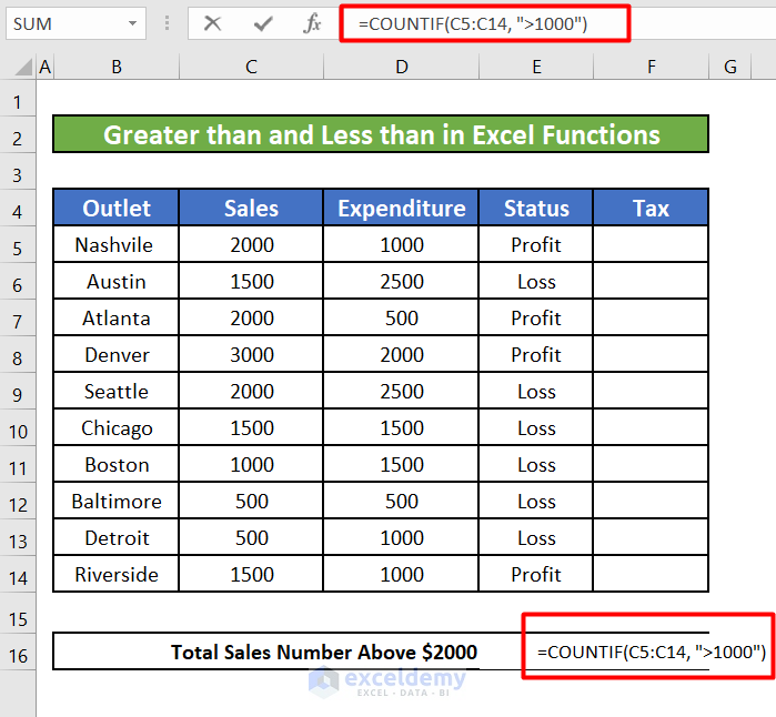
This function will count all the values in the Sales (C5:C14) column that is greater than 1,000.
Case 2.3 – Comparison Operators with the SUMIF Function
Steps:
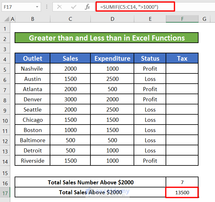
- To sum up all the sales amounts that are greater than $1,000, use this formula in cell F16.
=SUMIF(C5:C14, ">1000")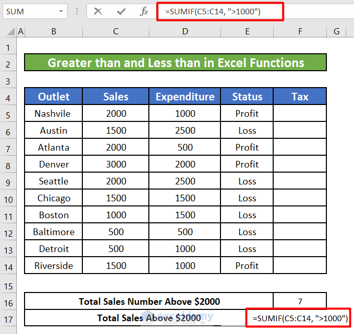
- The sum of all sales values above 1,000 is 13,500.
Read More: How to Apply ‘If Greater Than’ Condition In Excel
Method 3 – Comparison Operators in Excel Mathematical Operations
Steps:
- Consider the following IF function that calculates the tax to be paid by each outlet based on their sales amount.
=IF(C5>1500, C5*0.2, C5*0.1)This IF function will determine 20% as the tax rate for the sales amounts that are greater than $1,500 and multiply the tax rate with the sales amount. It will assume 10% as the tax rate for the sales amounts lower than $1,500.
- We can replace this IF formula with a formula constructed using only conditional operators.
=(C5>1500)*(C5*0.2)+(C5<=1500)*(C5*0.1)If a value in cell C5 is greater than 1500, then C5>1500 will be TRUE, which is implicitly converted to 1 for calculations. On the contrary, C5<=1500 will be FALSE and return 0. As in this example C5>1500, our formula can be interpreted like below:
1*(C5*0.2)+0*(C5*0)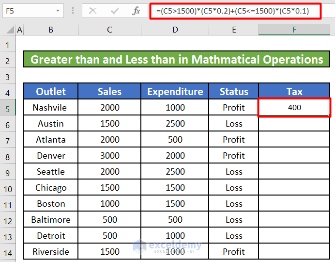
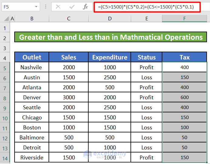
- If we drag the fill handle down, we will get the tax amounts for the rest of the sales values.
Method 4 – Comparison Operators in Excel Conditional Formatting
We will use conditional formatting with a greater than (>) conditional operator to find out the tax values greater than $300.
Steps:
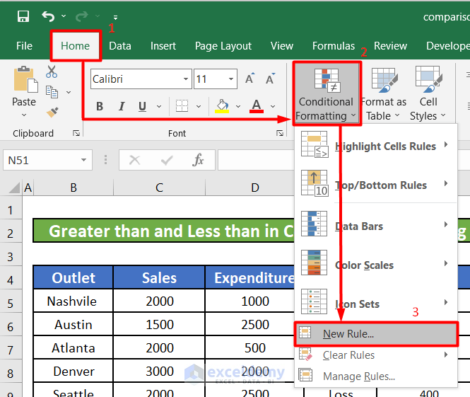
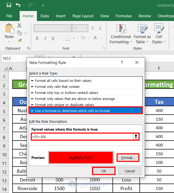
- Go to Conditional Formatting located in the Styles section under the Home ribbon.
- Select New Rule from the drop-down list.
- Select Use a formula to determine which cells to format from the Select a Rule Type list.
- Enter =F5>300 as the rule.
- Click on the Format button and select a color to highlight the cells. For this example, we have selected the Red color.
- Click on the OK button.
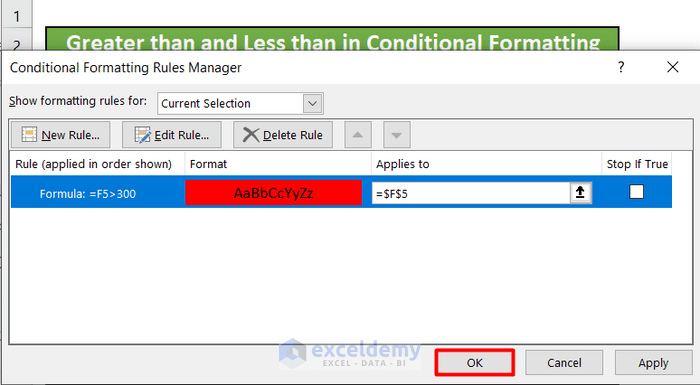
- A new dialog box titled Conditional Formatting Rules Manager will appear. Click OK.
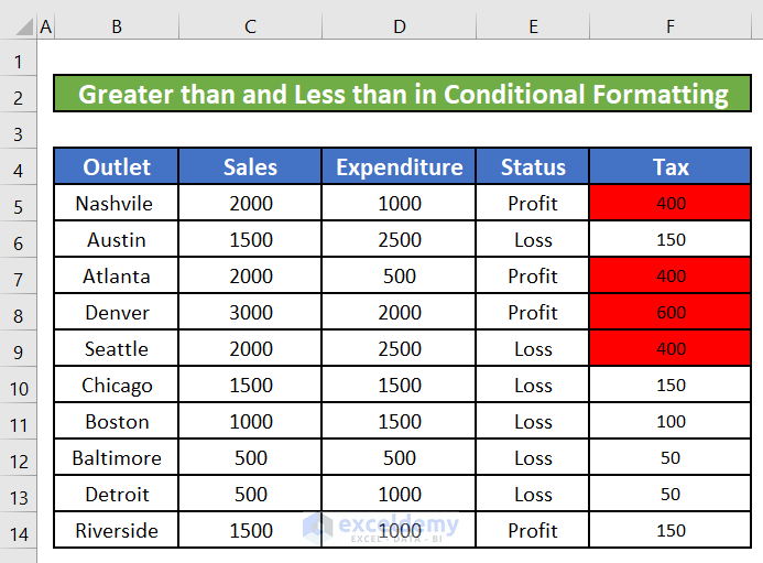
- Cell F5 will turn red as mentioned in the rule of conditional formatting as the value is greater than 300. Drag the fill handle to apply the conditional formatting to the rest of the cells in the Tax column.
Method 5 – Greater Than and Less Than Excel Comparison Operators with Text Values
When comparing text values, Microsoft Excel ignores their case and compares the values symbol by symbol, “a” being considered the lowest text value and “z” – the highest text value.
Steps:
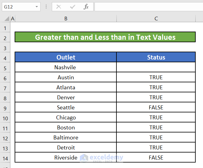
- We will compare the name of the first outlet (Nashville) with the rest of the outlets with the following formula in cell C6 under the Status column.
=$B$5>B6We have added two $ signs for cell B5. We are comparing the name of the first outlet with the rest of the outlets, so the first reference is absolute and won’t change when AutoFilling.
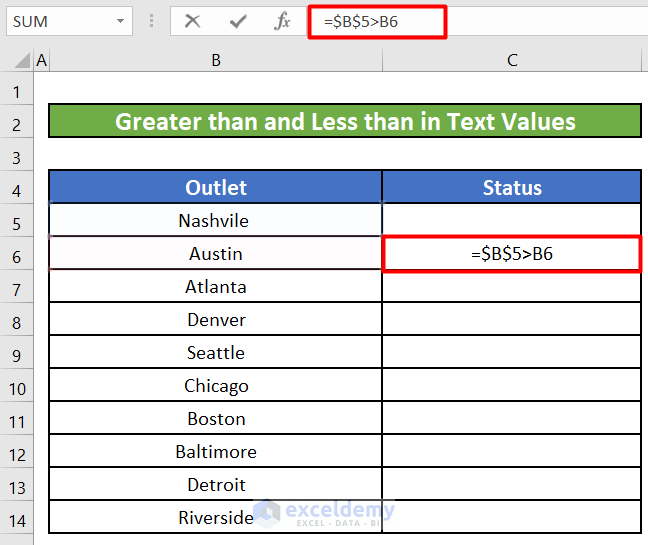
- Drag the fill handle to apply the formula to the rest of the cells.
Read More: Excel Boolean Operators: How to Use Them?
Download the Practice Workbook
Further Readings
- ‘Not Equal to’ Operator in Excel
- What is the Order of Operations in Excel
- Reference Operator in Excel
- How to Use Less Than Or Equal to Operator in Excel
<< Go Back to Excel Operators | Excel Formulas | Learn Excel
Get FREE Advanced Excel Exercises with Solutions!

