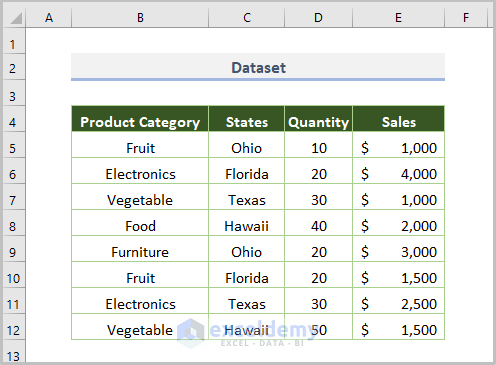
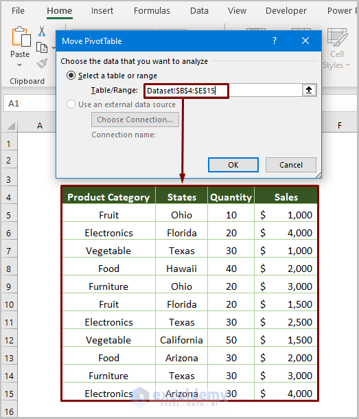
We have a dataset where the Product Category, Quantity, and Sales are given based on states.
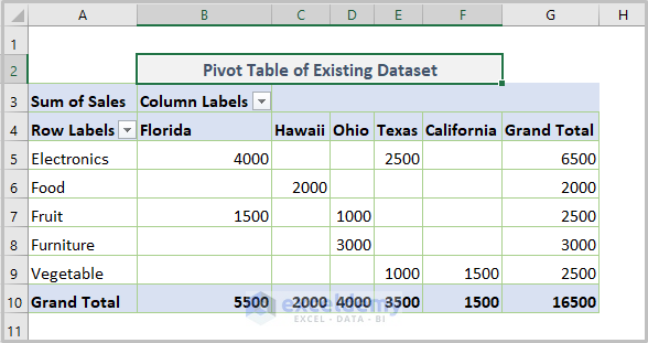
You can visit the How to create a Pivot Table article to insert a Pivot Table for the above dataset. We have created a Pivot Table as follows.
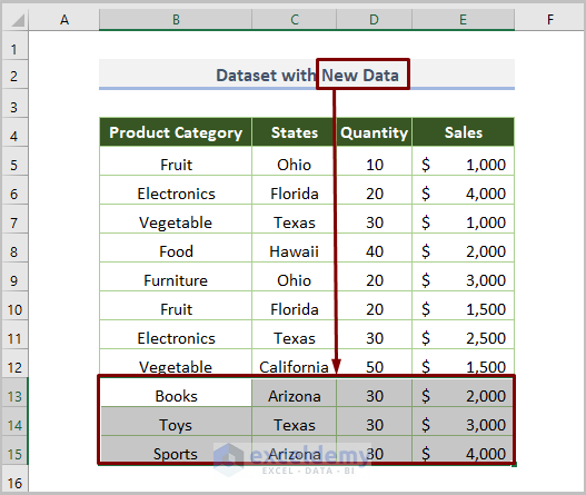
We need to add 3 more rows after the existing dataset. We’ll go over the most common issues and how to resolve them.
Issue 1 – New Data Is Not Included While Refreshing
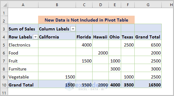
After adding that new data, we selected Refresh after right-clicking over a cell within the Pivot Table (keyboard shortcut Alt + F5) like the following screenshot.
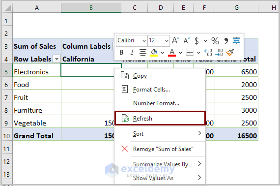
The Pivot Table does not update with the new data, which means the refreshing option is not working well.
Steps:
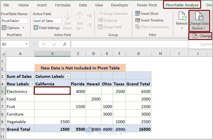
- Select a cell within the created Pivot Table.
- Click on Change Data Source… then select Change Data Source in the PivotTable Analyze tab.
- You’ll get a dialog box named Move PivotTable.
- Fix the new range of source data as $B$4:$E$15 and press OK.
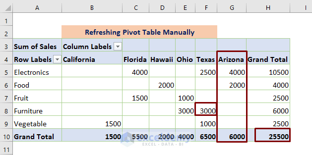
- We get a new column and updated values.
Issue 2 – PivotTable Shows an Error Message While Refreshing
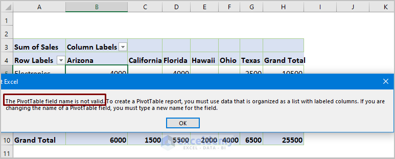
When trying to refresh the Pivot Table, Excel shows the error message “The PivotTable field name is not valid”.
The field States is empty.
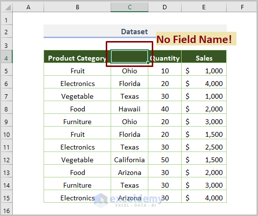
- To solve the problem, you need to add the field name.
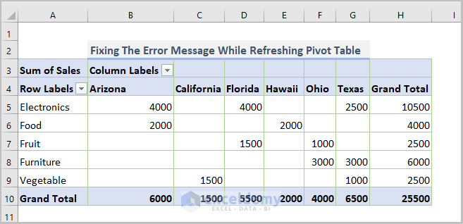
- When the field name States is added, pressing Refresh will work.
Read More: Automatically Update a Pivot Table When Source Data Changes in Excel
Issue 3 – Pivot Tables Overlapping
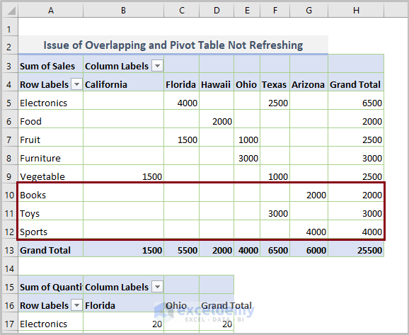
We’re adding more data into the table, which would extend the table by a few rows.

When trying to use the Refresh button, Excel shows an error message.
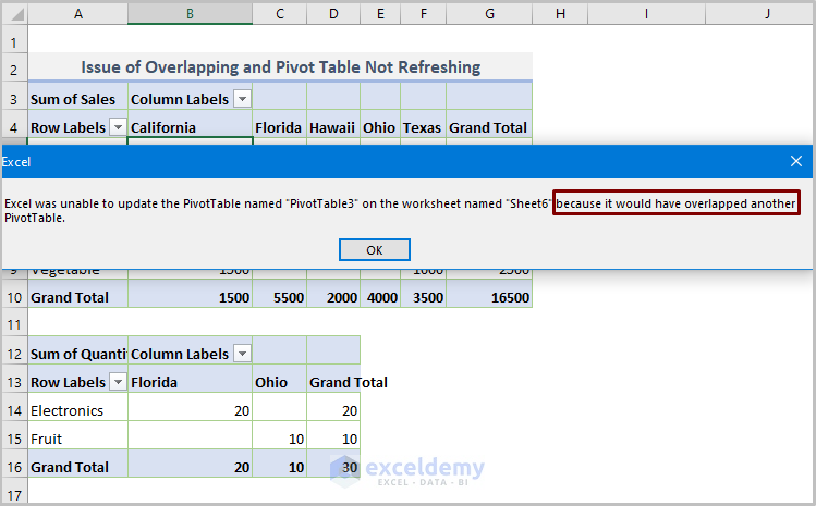
The cause of the problem is overlapping tables. There are two Pivot Tables in the current worksheet. If we were to refresh PivotTable1, it would extend into a different Pivot Table.
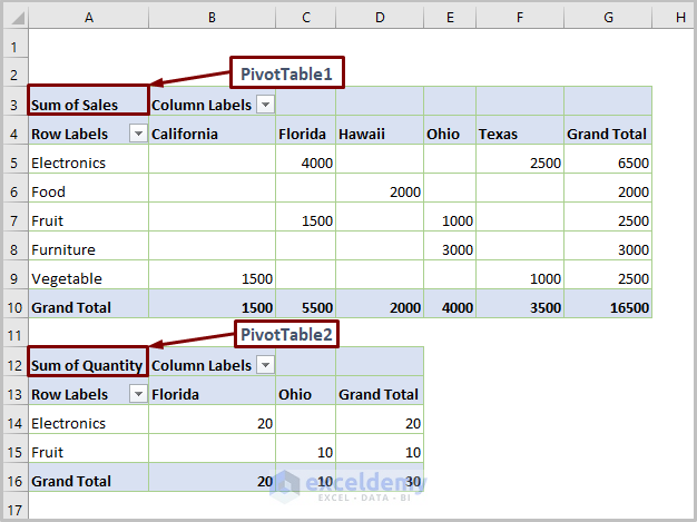
- Move the PivotTable2 to the cells below and refresh the PivotTable1.
- This solves the overlap problem.
Issue 4 – Pivot Table Not Refreshing When the Workbook is Opened
Functions like TODAY and NOW need to recalculate their results periodically.
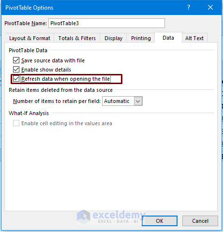
- Click PivotTable Analyze and select Options.

- Check the box for Refresh the data when opening the file.
Read More: How to Auto Refresh Pivot Table without VBA in Excel
Issue 5 – Format Changing While Refreshing the Pivot Table
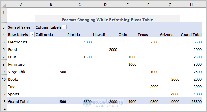
The column width is 12 and the cell border is available in the following Pivot Table.
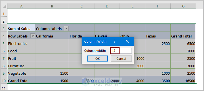
If we refresh the Pivot Table by clicking the Refresh button, you’ll see the following output where the column width and other cell formatting changes.
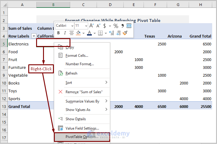
- Open the PivotTable Options by right-clicking after selecting a cell within the Pivot Table.
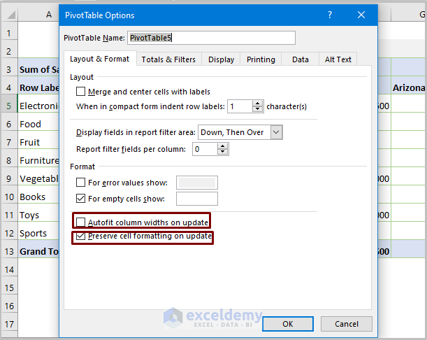
- In the PivotTable Options dialog box, uncheck the box for Autofit columns widths on update and check the box for Preserve cell formatting on update.
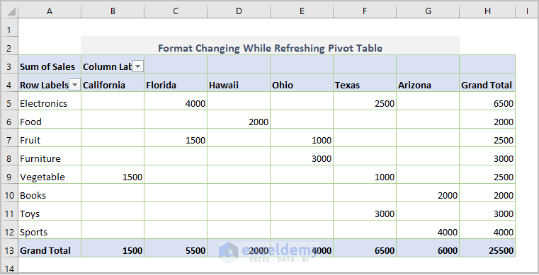
- Here’s the result.
Download the Practice Workbook


