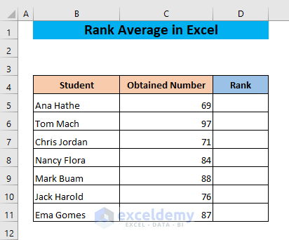
How to Rank Average in Excel (4 Common Scenarios)

We have a dataset with students and their scores, which we’ll use to rank the students.

Rank and Average in Excel

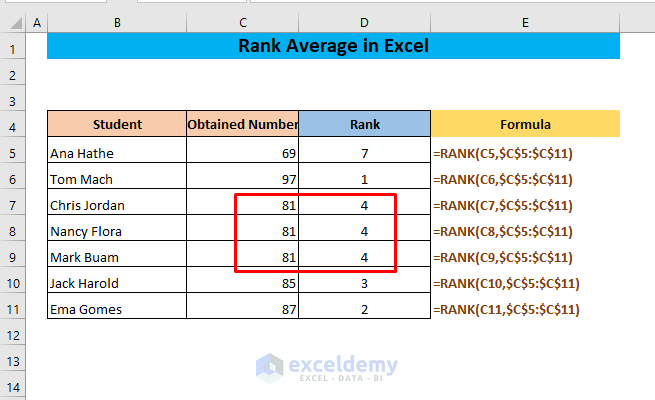
The RANK function is used to determine the rank or order of a number in a list. Using this function can rank the numbers of a list. But if there are two or more of the same values, the RANK function will display the same rank (the rank if the value is unique) for all the values.

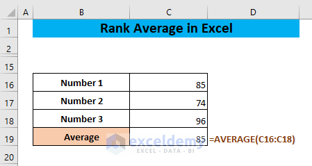
The AVERAGE function gives the average value of some numbers.

The RANK.AVG function works in the same manner as the RANK function, but it gives an average rank if there are two or more of the same values.

Read More: Excel Percentile Rank Inc vs Exc

Rank Average in Excel Simultaneously

The RANK.AVG function returns the rank of a number in a list of numbers: its size relative to other values in the list; if more than one value has the same rank, the average rank is returned.

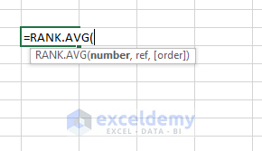
The syntax of this function is:

RANK.AVG(number, ref, [order])

Argument	Required/Optional	Explanation
number	Required	The numerical value whose rank will be determined in a list
ref	Required	An array or list that contains the numbers to rank against. The non-numerical entry of the list is ignored.
Order	Optional	The order of ranking, If empty or 0, the order will be descending. If 1, the order will be ascending.

This function is first available in Excel 2010.

Example 1 – Using Excel RANK-AVERAGE to Rank a List Based on a Value

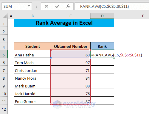
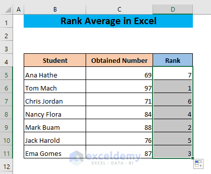
We have a dataset where the obtained scores of different students in a test are given.

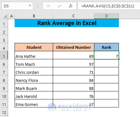
Use the following formula in cell D5:

=RANK.AVG(C5,$C$5:$C$11)

The function will determine the rank of the number in cell C5 in the list $C$5:$C$11.

Don’t forget to lock the range of the list.

Press ENTER.

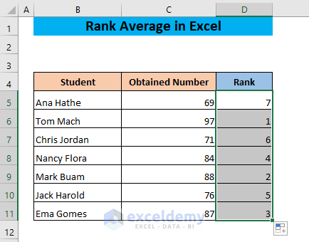
Drag the fill handle of cell D5 to the end of your dataset.

Example 2 – Ranking Duplicates with Excel Rank-Average Function

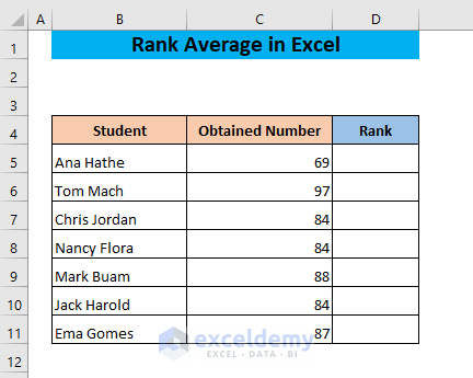
Let’s see what happens if there are duplicate values in the list. We have the following dataset where the number 84 appears three times.

Use the following formula in cell D5:

=RANK.AVG(C5,$C$5:$C$11)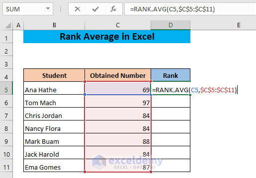

Hit Enter.

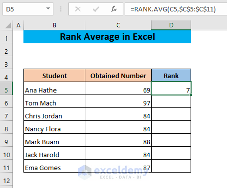
Drag down the fill handle.

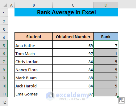
The formula gives the rank of the number 84 as 5. The number 84 appears three times. The previous number in the descending order is 87 whose rank is 3 and the next number in the descending order is 69 whose rank is 7. So, the three 84s occupy the 4th, 5th, and 6th positions since their average rank is 5.

Example 3 – Ranking in Ascending Order Using RANK-AVERAGE

Use the following formula in cell D5,

=RANK.AVG(C5,$C$5:$C$11,1)

The optional argument 1 indicates that the rank will be assigned in ascending order.

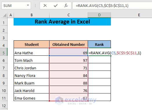
Hit Enter.

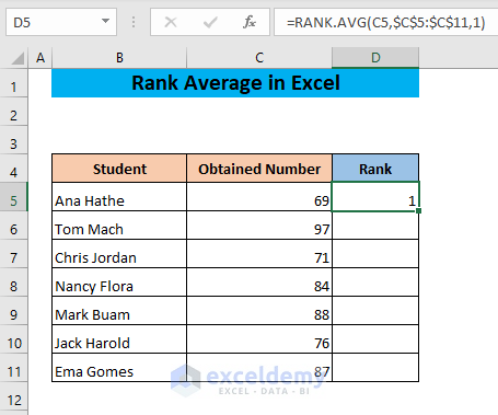
Drag cell D5 to the end of your dataset.

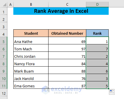
Example 4 – Ranking in Descending Order with RANK-AVERAGE

The RANK.AVG function ranks numbers in descending order by default. If you leave the optional argument empty or put 0, you will also get the rank in descending order.

Use the following formula in cell D5:

=RANK.AVG(C5,$C$5:$C$11,0)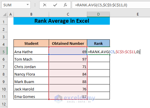

Press ENTER.

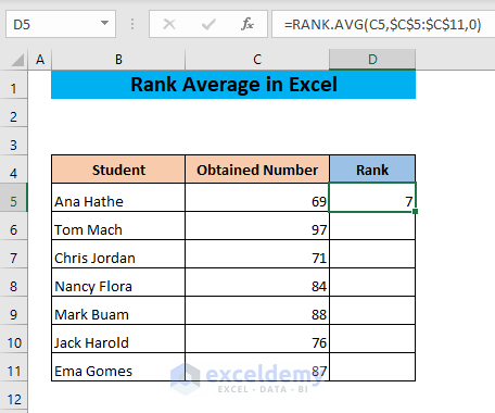
Drag the cell D5 to the end of your dataset.

Things to Remember

If the number is not in the range assigned as the ref, the function will return #N/A! Error.
If there is any non-numeric data in the list, it will be ignored by the RANK.AVG function.

Download the Practice Workbook

Rank Average.xlsx