How to Find a Cell That is Formatted as Text or Preceded by an Apostrophe
When we use an apostrophe before a number, or when values are stored as strings in our dataset, this error occurs. To find a cell that is formatted as text or preceded by an apostrophe, follow the steps below.
STEPS:
- Select an adjacent cell and enter the formula:
=ISNUMBER(B2)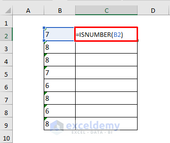
- Hit Enter.
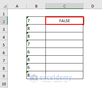
- Use the Fill Handle for all cells.
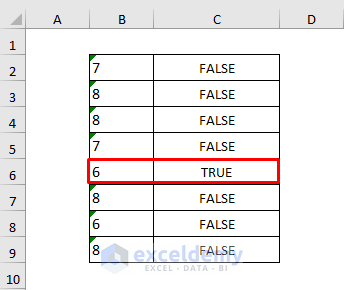
Here, only Cell B6 is stored as a number.
Excel Error: The Number in This Cell is Formatted as Text – 6 Solutions
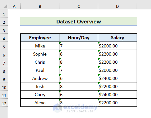
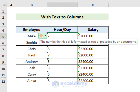
The sample dataset contains information about working hours and the salary of some employees. Here, the number values are showing an error.
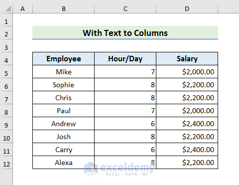
Solution 1 – Convert Text to Number with Text to Columns
If we select a cell and put the cursor on the smart tag, it will display an error like below.
STEPS:
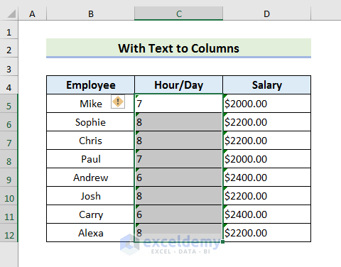
- Select all the cells of a single column. We have selected the cells of Column C.
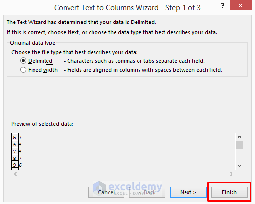
- Go to the Data tab and select Text to Columns. The Convert Text to Columns Wizard will appear.

- Click Finish from the Convert Text to Columns Wizard.
- The values of Column C will automatically convert to numbers and there will be no error.
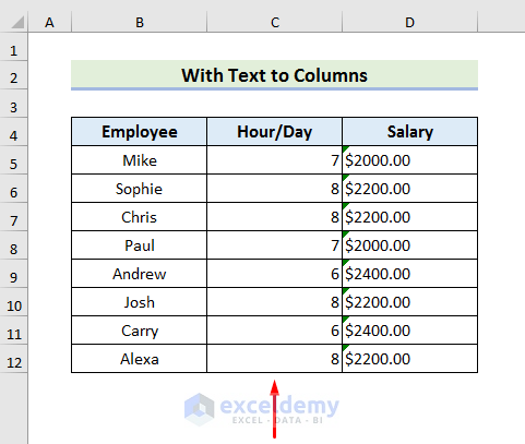
- Do the same for Column D.
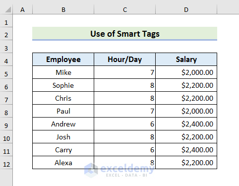
Solution 2 – Change Text to Number Using Smart Tags
If you select a cell that contains any errors, the smart tags icon highlighted below will appear automatically.
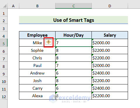
STEPS:
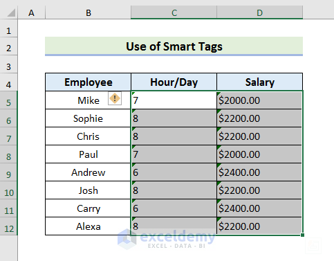
- Select the error cells first. We have selected Cell C5 to Cell D12.
- Click on the smart tags icon. A drop-down menu will occur.
- Select ‘Convert to Number’ from it.
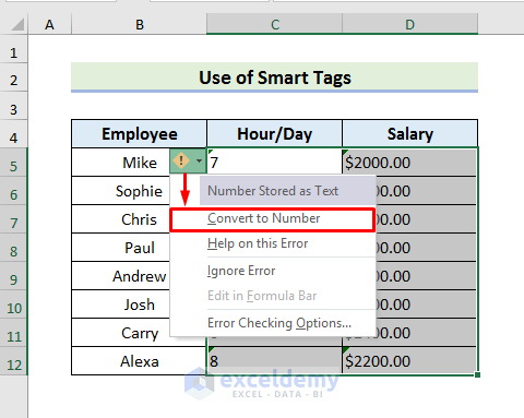
- The error has been fixed.
Solution 3 – Apply Paste Special to Convert Text to Number or Remove the Preceded Apostrophe
We can use the paste special option of Excel to convert text to numbers. There are two ways to use the paste special option.
In this first method, we will use the add operation.
STEPS:
- Select any cell in your dataset. We have selected Cell C14.
- Press Ctrl + C to copy the cell.
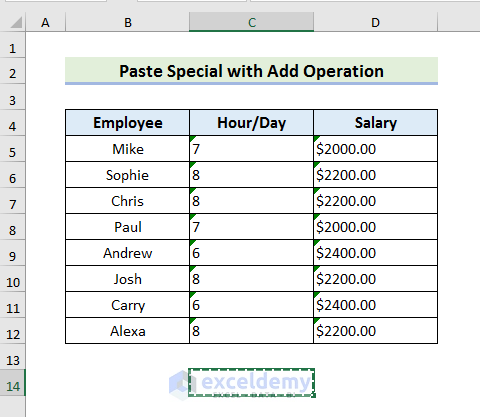
- Select the cells that have an error.
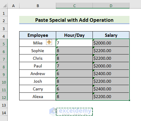
- Select Paste from the Home tab and select Paste Special from the drop-down menu.
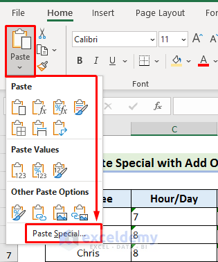
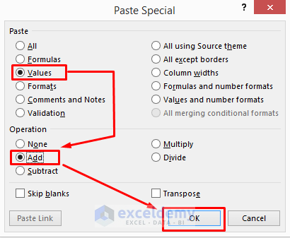
- The Paste Special window will open. Select Values and Add from the Paste Special.
- Click OK to proceed.
- The numbers will appear as below.
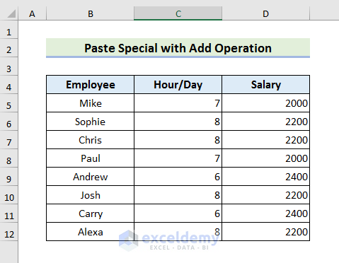
- To convert the Salary column into the desired format, select Column D.
- Go to the Home tab and select Currency from the Number Format box.

- Now the numbers are in the correct format.
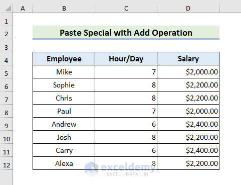
We can also use the multiply operation to fix this error.
STEPS:
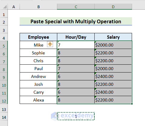
- Select any cell in your dataset and write 1. We have selected Cell C14.
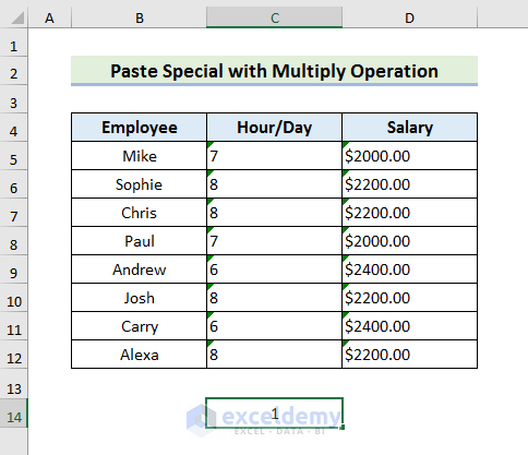
- Press Ctrl + C to copy the cell.
- Select the cells from where you want to remove the error.
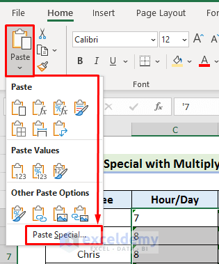
- Select Paste from the Home tab and select Paste Special from the drop-down menu. The Paste Special window will open.
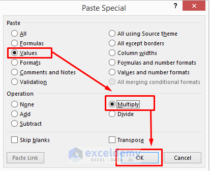
- Select Values and Multiply from the Paste Special window.
- Click OK to proceed.
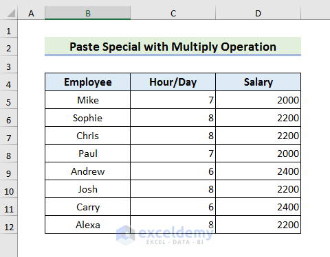
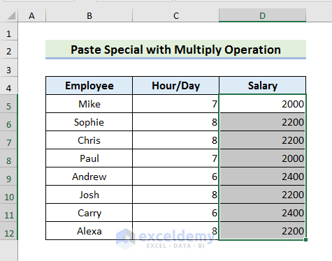
- After clicking OK, you will see the below results.
- To convert the Salary column into Currency, select Column D.
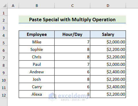
- Go to the Home tab and select Currency from the Number Format box.

- Now the numbers are in the correct format.
Solution 4 – Use of Value Function to Transform Text or a Cell Preceded by an Apostrophe to Number
STEPS:
- Insert a helper column as below.
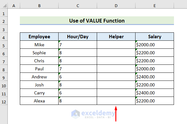
- Select cell D5 and enter the formula:
=VALUE(C5)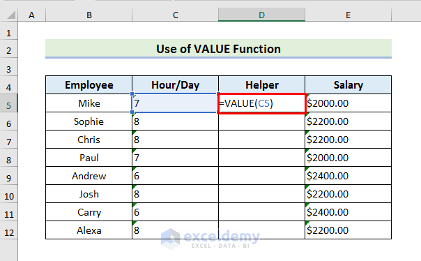
- Hit Enter.
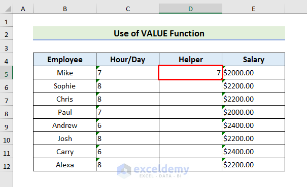
- Use the Fill Handle for the rest of the cells.
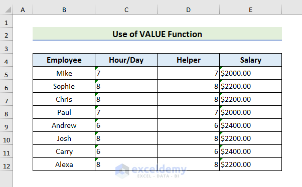
- Select the values of the helper column, press Ctrl + C to copy and select Column C.
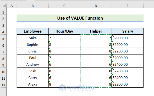
- Go to the Home tab and select Paste Special.
- Select Paste Values from the drop-down menu.
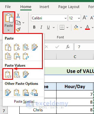
- There is no longer an error in Column C.
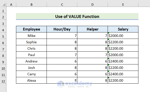
- Delete the helper column.
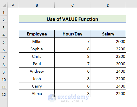
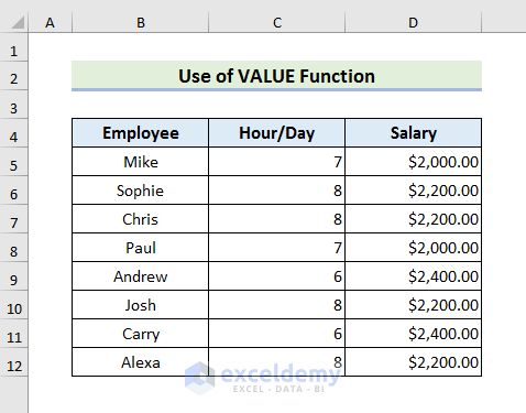
- You can change the Number Format to Currency to present the Salary column in the correct format.
Read More: [Fixed!] VALUE Error in Excel
Solution 5 – Insert Mathematical Operation to Change Text Cell to a Number
STEPS:
- Add an extra column.
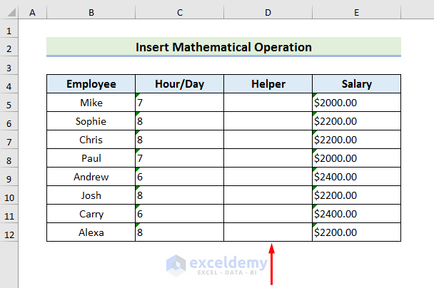
- Select cell D5 and type the formula:
=C5*1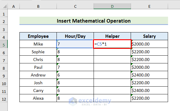
- Press Enter.
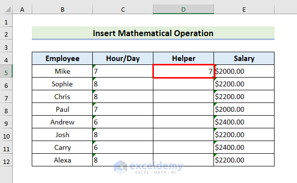
- Use the Fill Handle to see results in all cells.
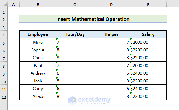
- Delete the Helper column.
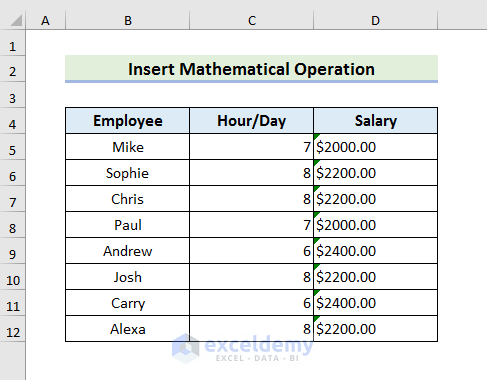
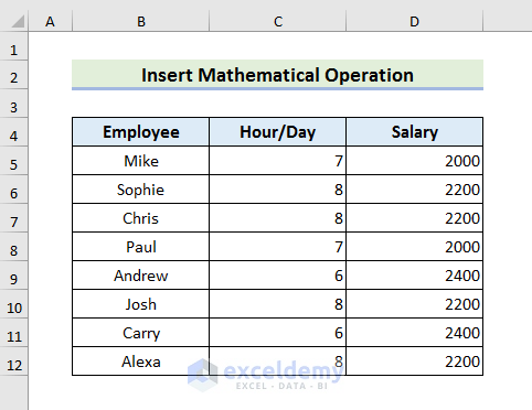
- Repeat the steps for Column D and you will see results like below.
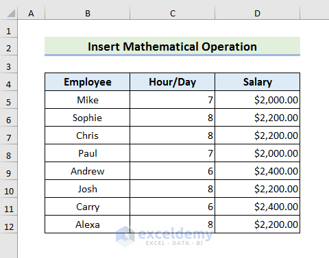
- Change the Number Format to Currency to see the desired result.
Solution 6 – Apply VBA to Convert Text to Number
STEPS:
- Go to the Developer tab and select Visual Basic. The Visual Basic window will appear.

- Go to Insert and select Module.
- Type the code in the Module window.
Sub Convert_to_Number()
With Worksheets("VBA").Range("C:C")
.NumberFormat = "General"
.Value = .Value
End With
With Worksheets("VBA").Range("D:D")
.NumberFormat = "General"
.Value = .Value
End With
End Sub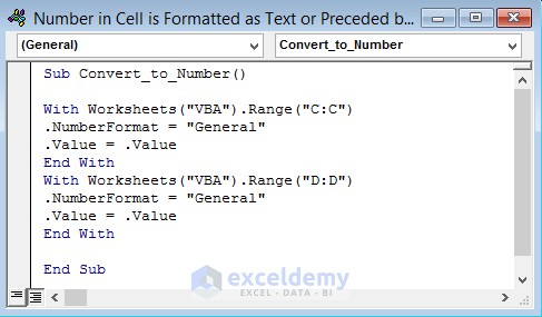
Here, we have selected Column C using Range and changed the number format to general. We have repeated the same thing for Column D.
- Press Ctrl + S to save the code.
- Select Macros from the Developer tab. The Macro window will appear.

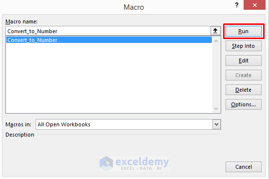
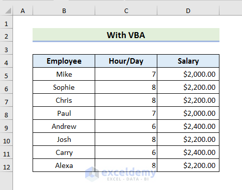
- Select the code from the Macro window and Run it.
- You will see results like below.
How to Ignore ‘The Number in This Cell is Formatted as Text or Preceded by an Apostrophe’ Error in Excel
To ignore any error, select a cell that has an error and then select the smart tags option. You will find the ‘Ignore Error’ option in the drop-down menu.
Download Practice Book
Download the practice book here.
Related Articles
- How to Remove #DIV/0! Error in Excel
- How to Calculate Mean Squared Error in Excel
- How to Calculate Root Mean Square Error in Excel
- How to Remove Value Error in Excel
- [Fixed!] NUM Error in Excel
<< Go Back To Errors in Excel | Learn Excel
Get FREE Advanced Excel Exercises with Solutions!

