Errors in Excel and Their Meaning (15 Different Errors)

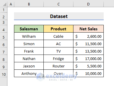
We’re going to use a sample dataset to show most common errors. The following dataset represents the Salesman, Product, and Net Sales of a company.

Errors in Excel and Their Meaning: 15 Different Errors

Formula Errors in Excel and Their Meaning

Type 1 – ##### Error

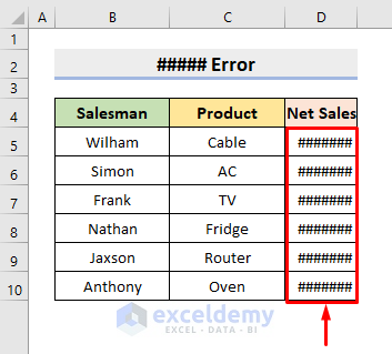
The most common error in Excel is the ##### error. This is not a formula-based error. It happens due to the width of the column being too small to show the entire cell value.

In the following dataset, column D has the ##### error.

Solution:

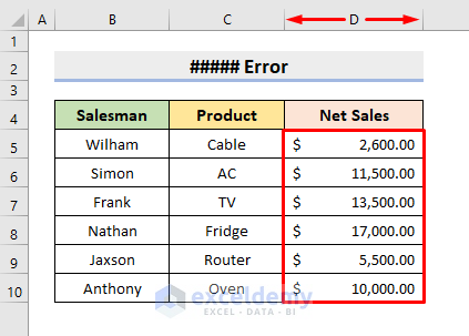
Expand the column width by dragging the boundary on the right side and you’ll get to see the values properly.

Type 2 – #DIV/0 Error

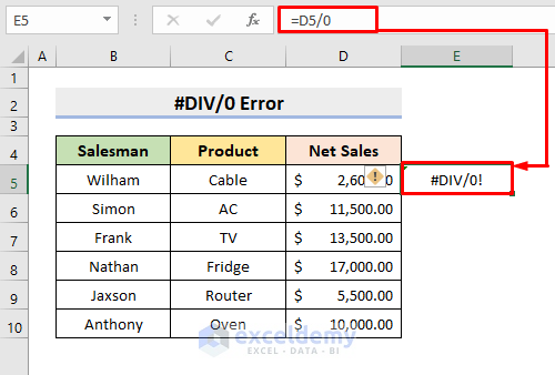
#DIV/0 error shows up as we divide any number or cell value by 0.

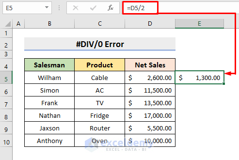
In cell E5, we attempt to divide D5 by 0, so it shows #DIV/0!.

Solution:

Divide D5 by any value other than 0, and the error won’t occur.

Type 3 – #NAME? Error

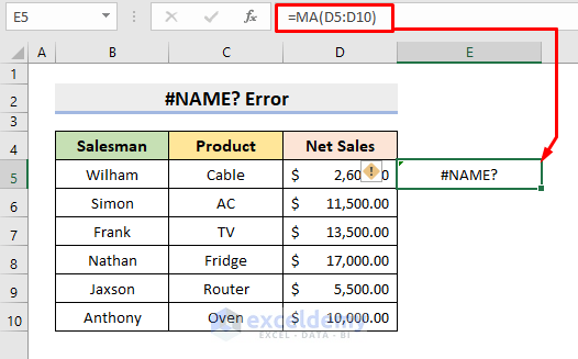
If we make a spelling mistake in writing the function name, Excel shows this error. This problem happens whenever Excel isn’t able to recognize the text in the formula.

In the below dataset, Excel can’t recognize the formula in cell E5.

Solution:

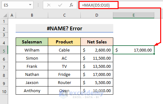
Instead of MA in the formula, type MAX and you’ll get the accurate value.

Type 4 – #N/A! Error

This error arises when the formula or a function in the formula fails to find the referenced data. It mostly occurs with lookup functions.

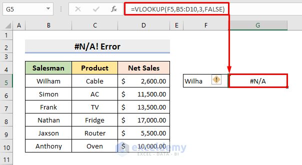
In the given dataset, we’ll try to look for the cell F5 data in the range B5:D10. But, #NA! error occurs. The F5 cell value doesn’t exist in the range.

Solution:

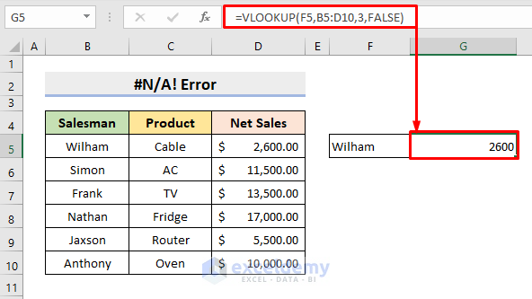
Input the reference data correctly. In this example, type Wilham in cell F5. It’ll return the Net Sales amount of Wilham.

Type 5 – #REF! Error

The #REF! Error is also a common error that arises when we accidentally delete any row or column that we have referenced in the formula. It can also arise when we copy and paste formulas with relative references to a different location.

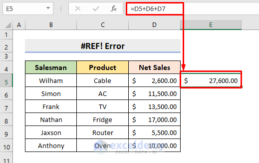
In this case, we add the cells D5, D6, and D7 in cell E5.

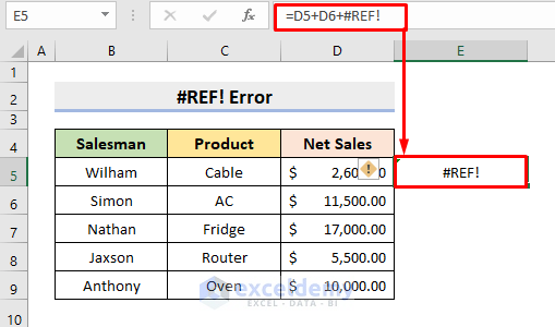
But, as we delete the 7th row, the #REF! Error occurs in cell E5.

Solution:

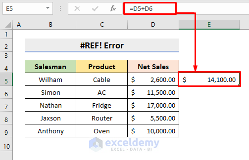
Type the formula again for cells D5 and D6. As a result, you’ll get the precise value.

Read More: How to Fix #REF! Error in Excel

Type 6 – #VALUE! Error

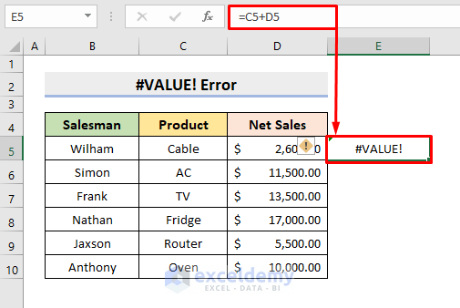
When a value isn’t a valid type, or when we use a wrong type of function argument, the #VALUE! Error occurs.

In this example, we try to add cells D5 and C5 to cell E5. But, as the data type is not the same for the two cells, the error arises.

Solution:

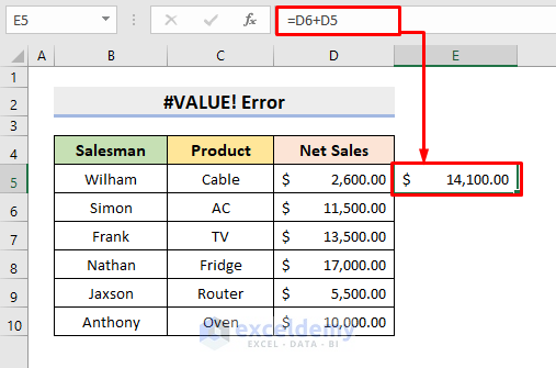
To avoid this error, input the same type of data type in the formula. Here, instead of C5, type D6, and it’ll return a result.

Type 7 – #NUM! Error

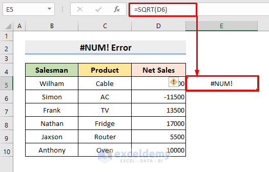
This error arises when the formula contains invalid numeric data in that operation and the calculations become impossible.

The below dataset attempts to find the square root of cell D6. But, D6 is a negative number and the function SQRT won’t work with negative numbers. Thus, the #NUM! Error shows up.

Solution:

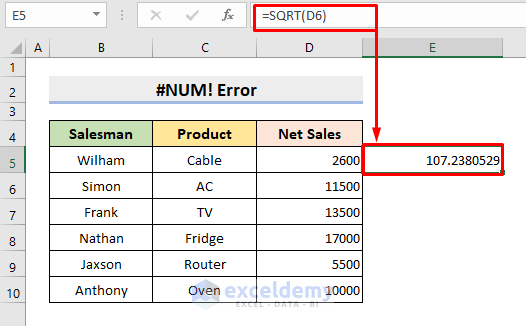
Remove the minus from cell D6 value and it’ll immediately return the square root.

Type 8 – #NULL! Error

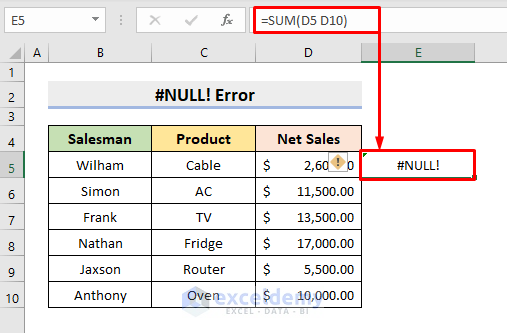
#NULL! error occurs when we place a Space instead of a Comma or a Colon in the function argument.

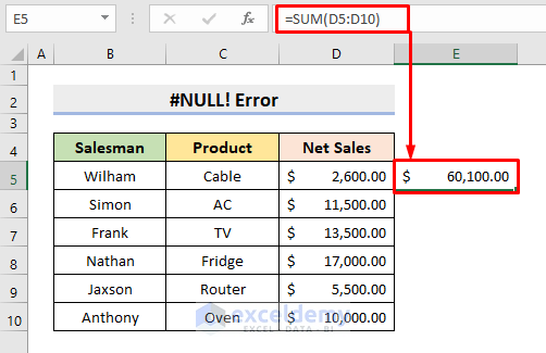
In the following dataset, we used the SUM function to add the values in the range D5:D6. Since we input a space instead of a colon between D5 and D10, the #NULL! Error occurs.

Solution:

Place a colon between D5 and D10 and you’ll get the sum result.

Type 9 – Circular Reference Error

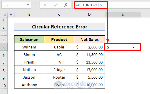
When we reference the same cell in which we are writing the formula, the Circular Reference Error occurs.

In cell E5, we wrote a formula, but E5 is also a reference data in the argument. As soon as we press Enter, ‘–’ shows up.

Solution:

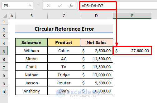
Remove E5 from the formula and the error will disappear.

Type 10 – #SPILL! Error

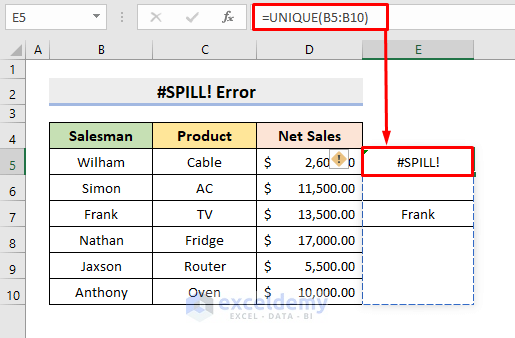
This error arises whenever a formula gives out a spill range that runs into a cell that already contains a value.

We used the UNIQUE function to pull out the unique names in column B into a spill range starting in cell E5. But, E7 already has a value. Thus, the #SPILL! Error shows up.

Solution:

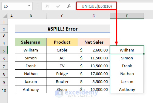
Delete the cell value in E7. The formula will return the unique names.

Type 11 – #CALC! Error

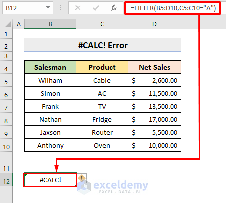
If a formula runs into a calculation error with an array, the #CALC! Error arises.

In this FILTER function, it asks for A from the range C5:C10 which doesn’t exist. Hence, the error shows up.

Solution:

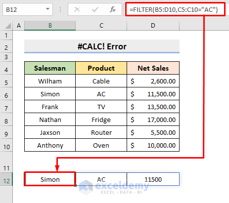
Replace A with AC and it’ll return the result.

File Errors in Excel and Their Meaning

Type 1 – “The file is corrupt and cannot be opened” Error

If you upgrade your Excel, it’s very likely that you’ll see this error message. Change the settings given below to solve the problem.

STEPS:

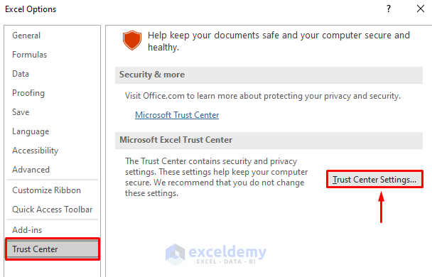
• Click the File tab and select Options.
• Select Trust Center from the Excel Options window.
• Select Trust Center Settings.

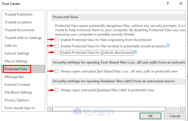
• A new window will pop out.
• In Protected View, uncheck all the options and press OK.

Type 2 – “Excel cannot open the file ‘(filename)’.xlsx” Error

If the file you are trying to open is not compatible with the Excel version and if it is corrupted or damaged, this error message shows up.

STEPS:

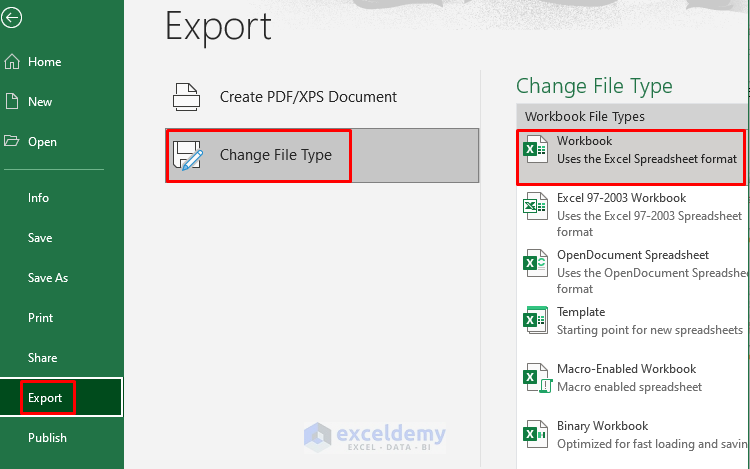
• Open Excel and select the tab File.
• Select Export, and then select Change File Type.
• Change the file format and save the new file.

Type 3 – “The document caused a serious error the last time it was opened“ Error

If the Excel file is included in the list of disabled files, it’ll cause serious errors.

STEPS:

• In Excel, select the File tab.
• Select Options.
• In the Add-ins tab, select COM Add-Ins in the Manage box.
• Click Go.

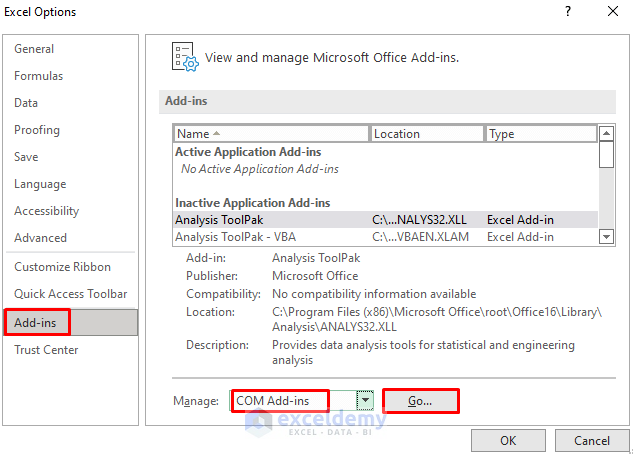
• A dialog box will pop out. Uncheck all the boxes in the Add-ins available section.
• Press OK.

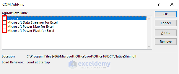
• Now, restart the application to finish the setup.

Type 4 – “There was a problem sending the command to the program” Error

This error message arises when the process running in the Excel file doesn’t let Excel close.

STEPS:

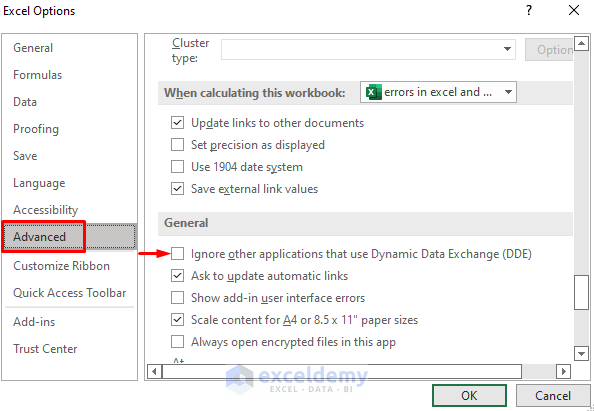
• Select the File tab and choose Options.
• Select Advanced.
• In the General section, uncheck the Ignore other applications that use Dynamic Data Exchange (DDE) box.
• Press OK.

Functions to Check Excel Errors

Type 1 – The ISERROR Function

We can use the ISERROR function to check if there would be any error in our applied function.

In the below dataset, cell E5 contains a formula which can produce an error.

STEPS:

• Use this formula:

• Press Enter and it’ll return the text Error.

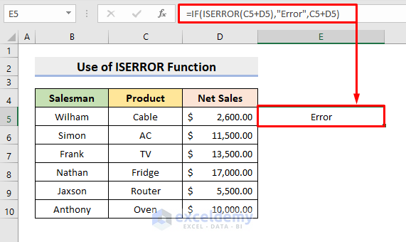
The IF function finds out whether a certain condition is met or not. In this example, the condition is the ISERROR function. If the condition is satisfied, it’ll return an Error. The ISERROR function checks to see if there is an error in C5+D5. Since C5 is a text, the formula won’t work and it’ll return an Error.

Type 2 – AGGREGATE Function

The AGGREGATE function calculates ignoring any error values.

We want to find the sum of the range D5:D10. If we use the SUM function in cell E5, it’ll return the error as we have an error value in cell D6.

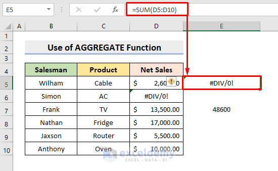
STEPS:

• In cell E7, use the formula:

• Press Enter and it’ll return the result.

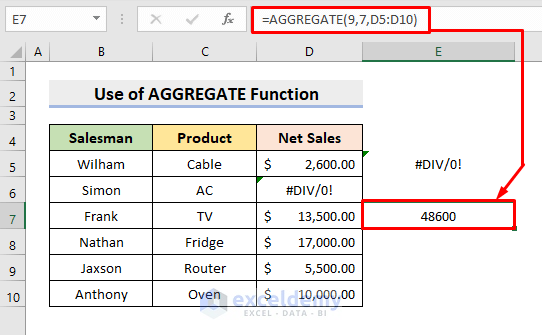
NOTE: 9 is the function number for SUM, 7 is the option to Ignore hidden rows and error values, and D5:D10 is the applicable range.

Download the Practice Workbook

Errors in Excel: Knowledge Hub

<< Go Back To Learn Excel