How to Select Cells with Certain Value in Excel (5 Methods)

Dataset Overview

Occasionally, we need to locate and highlight cells with specific values in an Excel spreadsheet. Since Excel typically contains a variety of data entries, there are instances when we specifically want to identify and select certain values. For example, consider a dataset that includes information on Products, Quantities sold, and Prices. We may want to highlight cells containing specific values within any column. In this article, we explore how to achieve this using built-in Excel features and VBA macros.

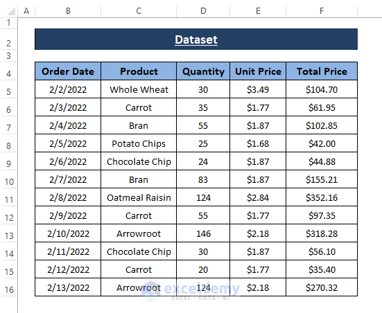
Method 1 – Using Excel’s Find Feature

Navigate to the Home tab.
From the Editing section, choose Find & Select and then select Find.

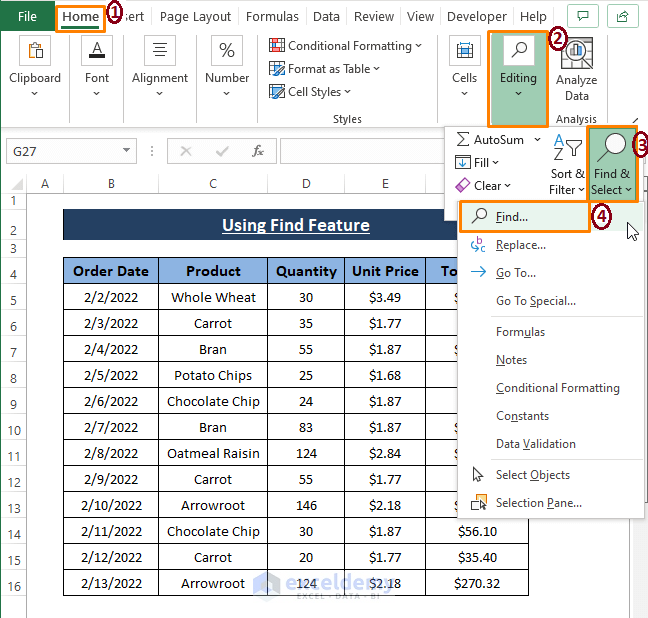
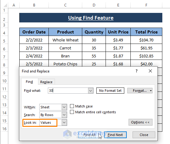
The Find and Replace window will appear. Ensure you are in the Find section.
Leave other options unchanged, but specifically choose Values as the Look in option.
In the Find what dialog box, type the desired value (e.g., 30).
Click Find All.

All cells containing the specified value (e.g., 30) will be listed below the Find and Replace window.
Press CTRL+A to select all the found cells at once.
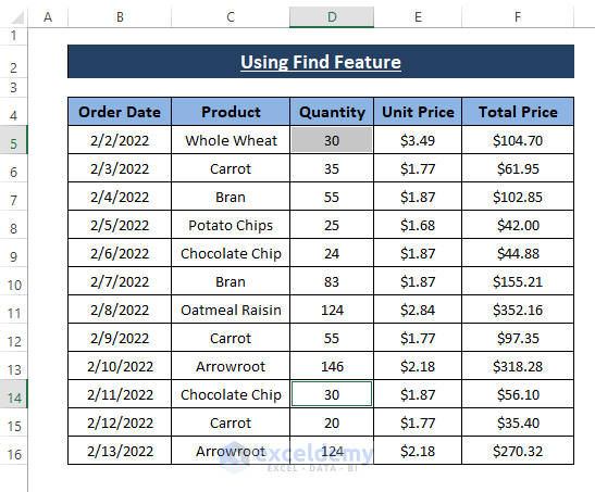
In your dataset, you’ll see the 2 cells containing the exact value 30 are now selected.

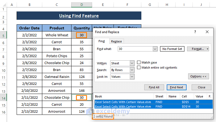
Click Close in the Find and Replace window to view the selected cells.

Method 2 – Using Conditional Formatting

Conditional Formatting is a powerful feature in Excel that allows you to highlight cells containing specific values. It provides various options for selecting or emphasizing cells based on their content type (whether text or numeric). When our goal is to pinpoint particular cells with specific values, we can utilize the ‘between’ or ‘equal to’ options to achieve this.

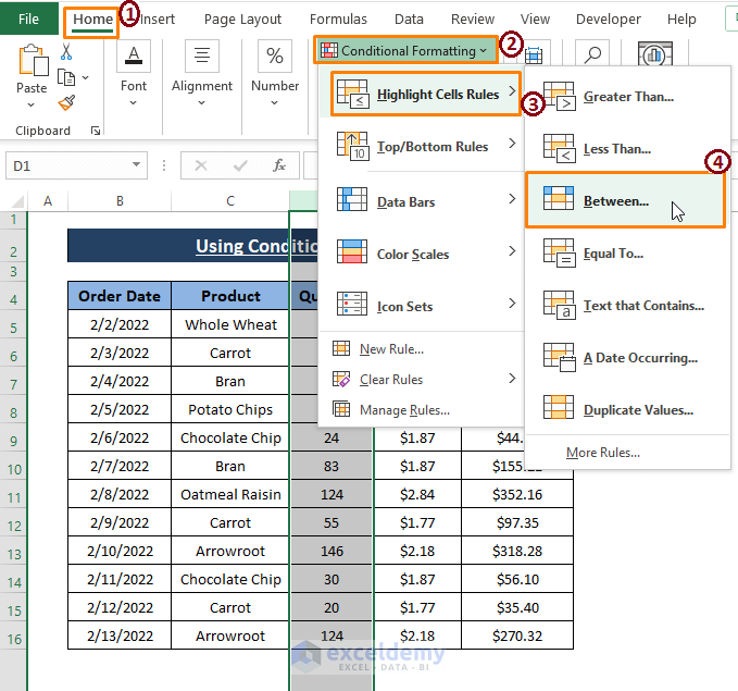
Select a range or column (e.g., the Quantity column).
Go to the Home tab, then click on Conditional Formatting in the Style section.
Choose Highlight Cells Rules and then select Between.

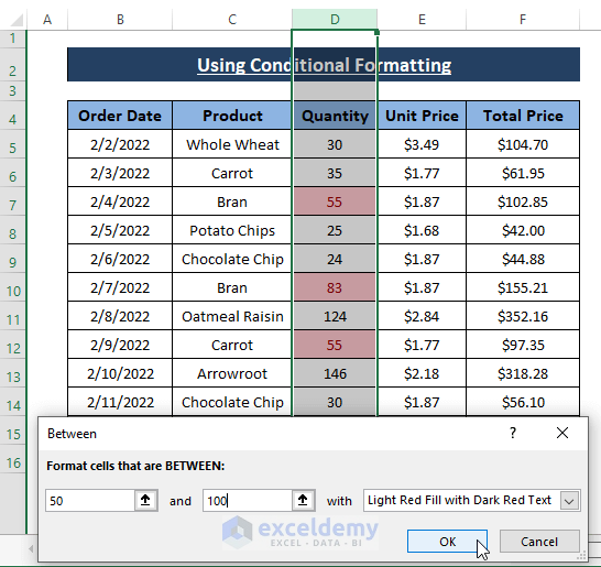
In the Between window, enter the 2 values (e.g., 50 and 100) that you want to use for selecting values in between.
Click OK.

Excel will apply Conditional Formatting to cells containing values between 50 and 100, as shown in the screenshot below.

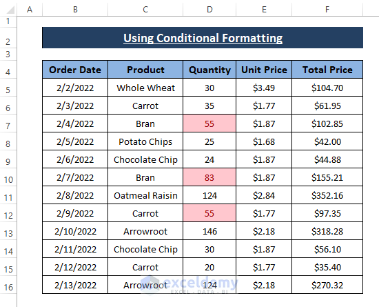
You can also customize the cell highlight color if desired. Additionally, you can use the same approach to select cells containing values between any other specified numbers.

Select Cells Containing Exact Value

Conditional Formatting offers various options, including finding and highlighting cells with equal values within a column or dataset.

Go to the Home tab.
Select Conditional Formatting from the Style section.
Choose Highlight Cells Rules and then click on Equal To.

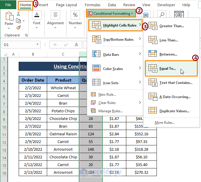
In the Equal To window, enter the desired value (e.g., 30) in the Format cells that are Equal To dialog box.
Click OK.

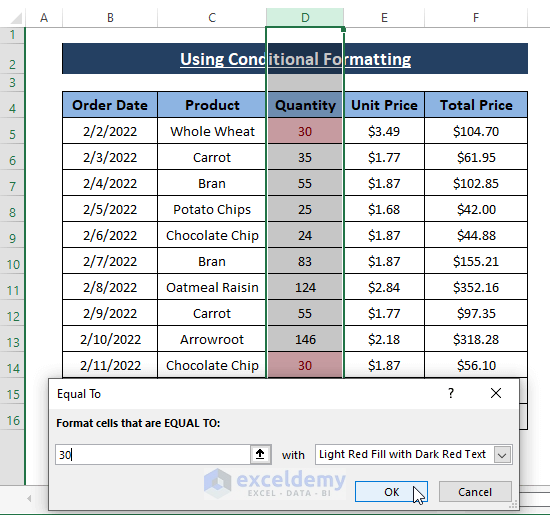
You’ll see a similar selection of cells as before, containing values equal to 30. Feel free to assign any other value to select specific cells within your dataset and apply color formatting using conditional formatting.

Method 3 – Using the Custom Filter Feature

In the previous method, we utilized Conditional Formatting to select cells with values between two specified numbers. Now, let’s explore a different approach using the Custom Filter feature.

Go to the Home tab.
From the Editing section, select Sort & Filter, and then choose Filter.

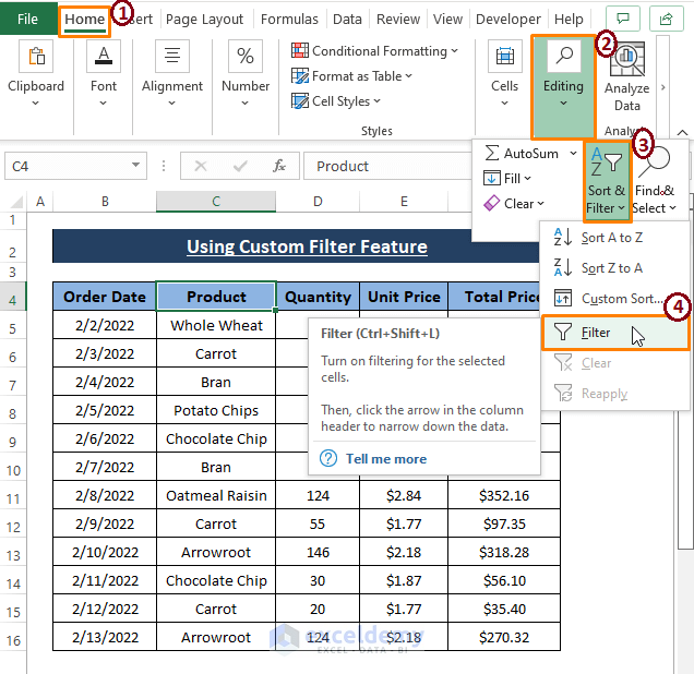
The Filter icon will appear in the column headers, as shown in the image.
Click on the Filter icon for the “Quantity” column.
Select Number Filters, and then choose Custom Filter.

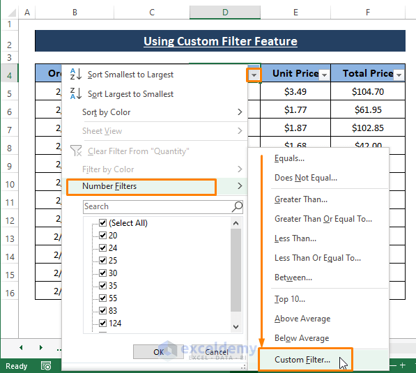
In the Custom AutoFilter window, set the following conditions:
- Choose Is greater than or equal to.
- Enter 50 as the value.
- Choose Is less than or equal to.
- Enter 100 as the value.
Click OK.

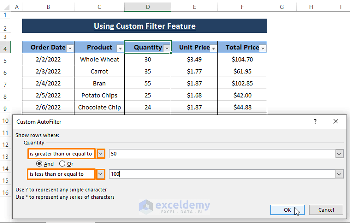
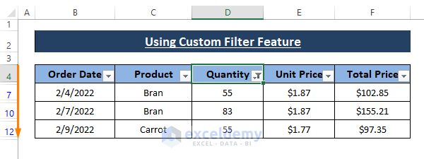
As a result, Excel will filter the values between 50 and 100 in the Quantity column. Rows containing values outside this range will be hidden.

Method 4 – Using “Go to Special” Feature

Suppose you have a dataset in Excel, and you want to select all the values within it. The Go to Special feature can help you achieve this.

We aim to select all the values present within the dataset. Based on the screenshot provided, we can identify the following columns as containing values:

Order Date
Quantity
Unit Price

Additionally, there are other columns with different data types:

The Product column contains text.
The Total Price column is a formula column.

Here’s how: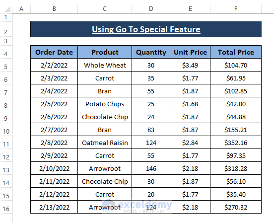

Select the Entire Dataset:
- Highlight the entire dataset that you’re working with.

Access the “Go to Special” Command:
- Go to the Home tab in the Excel Ribbon.
- Under the Editing section, click on Find & Select.
- From the dropdown menu, choose Go To Special.

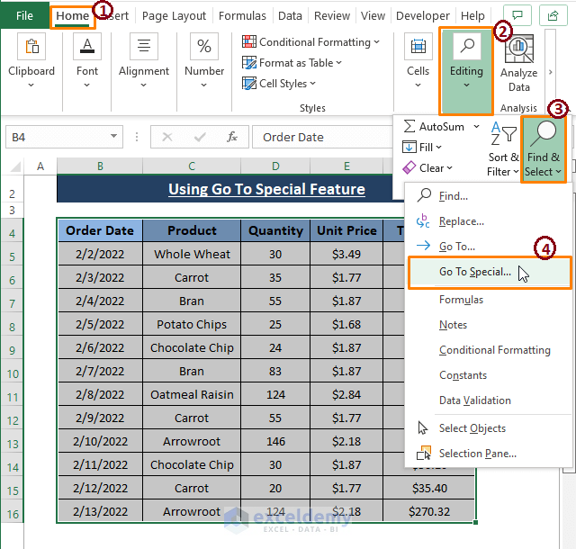
Configure the “Go to Special” Dialog Box:
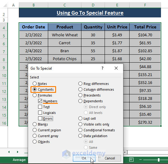
- The Go to Special dialog box will appear.
- Select the Constants option from the available choices.
- Make sure to unselect other options like Text, Logicals, and Errors, leaving only Numbers checked.

Click OK:
- Click the OK button.
- Excel will now highlight all the cells containing values within your dataset.

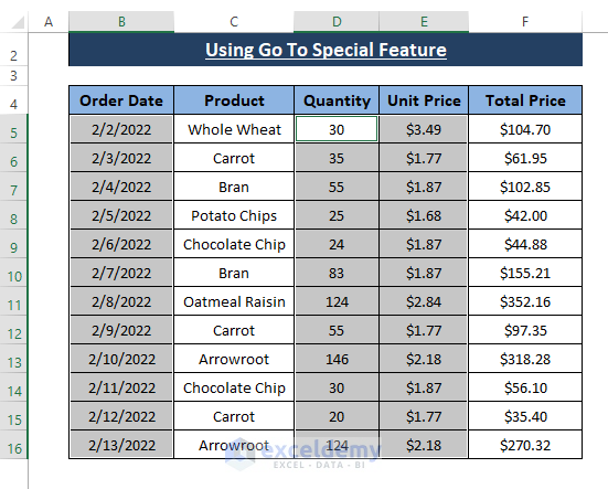
This method is particularly useful when dealing with datasets that have occasional value entries in cells. By following these steps, you can efficiently select the desired value cells using the “Go to Special” feature in Excel.

Method 5 – Using VBA Macro to Select Cells with Specific Values

VBA macros can be powerful tools for automating tasks in Excel. In this case, we’ll create a macro that selects cells containing a specific value within a given worksheet. Let’s walk through the steps:

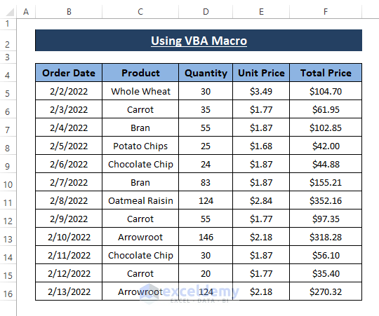
Press ALT + F11 together to open the Microsoft Visual Basic for Applications (VBA) window.
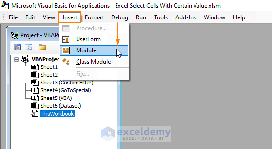
In the VBA window, go to the Insert menu (from the Toolbar) and select Module.
This will create a new module where we can enter our macro code.

Paste the following VBA macro code into the module:

Sub Selecting_specific_value()
Dim wrkSheet As Worksheet
Dim CellSelection As Range
Dim wrkcell As Object
Set wrkSheet = Worksheets("VBA")
For Each wrkcell In wrkSheet.UsedRange.Cells
If wrkcell.Value = 30 Then
If CellSelection Is Nothing Then
Set CellSelection = Range(wrkcell.Address)
Else
Set CellSelection = Union(CellSelection, Range(wrkcell.Address))
End If
End If
Next
CellSelection.Select
End Sub

Replace VBA with the actual name of your worksheet if it’s different.

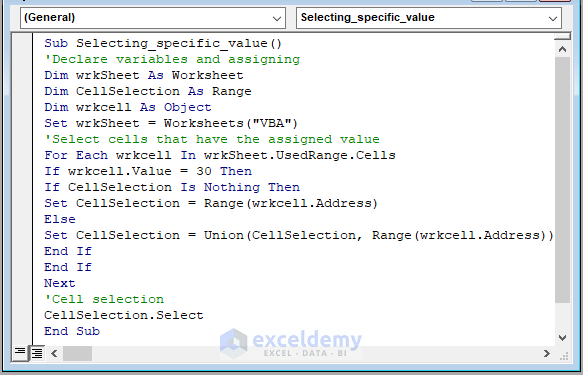
Press F5 to run the macro.
Return to your Excel worksheet, and you’ll see that cells containing the specific value (in this case, 30) are now selected.

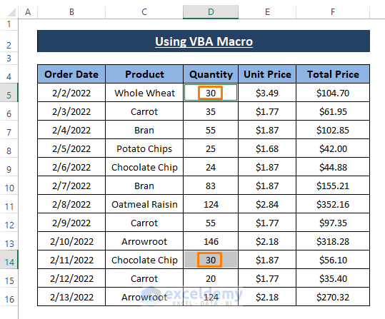
You can customize the value (30 in this example) in the macro to match your specific criteria. Additionally, feel free to assign any worksheet name to select cells from. VBA macros provide flexibility and efficiency for working with data in Excel.