How to Remove Blank Cells from a Range in Excel (9 Methods)

We have a data range (B4:E12) that contains sales data for several electronic products (Date-wise). You can delete blank cells manually by selecting them one by one (see screenshot), which seems time-consuming when the data range is large. We will show you 9 methods to remove blank cells in Excel.

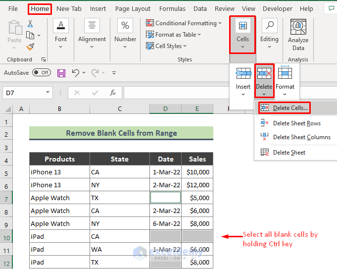
Method 1 – Excel ‘Go To Special’ Option to Delete Empty Cells from a Range

Steps:

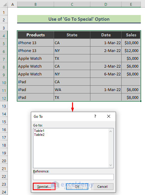
• Select the range (B4:E12) of data and press F5 or Ctrl + G to bring the Go To dialog box.
• Press Special from the dialog box.

• The Go To Special dialog box appears. Choose Blanks from the available options and press OK.

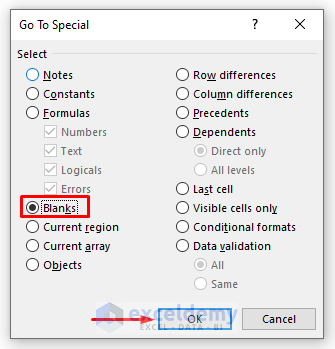
• All the blank cells in the range are highlighted.
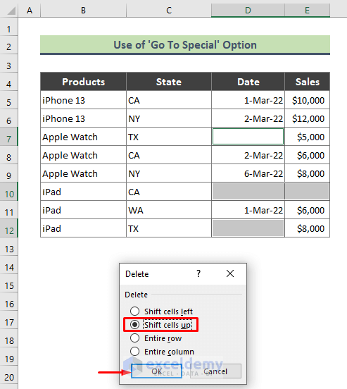
• Press Ctrl + – (minus) to bring up the Delete dialog.
• Choose your delete options. We have chosen Shift cells up.
• Press OK. We deleted the blank cells and moved non-empty cells up.

• Here is our result.

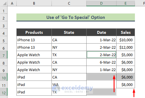
⏩ Note:

• Be careful while choosing the delete options from the Delete dialog. Choosing the wrong delete option will mess up your data range.
• You can bring the Delete dialog by right-clicking on the selection or following the path: Home > Cells > Delete > Delete Cells.

Read More: How to Delete Blank Cells and Shift Data Up in Excel

Method 2 – Remove Blank Cells from a Range Using the Filter Option

Steps:

• Select the range and press Ctrl + Shift + L to apply Filter on it.
• As the Filter option is applied, the drop-down arrows will show up.

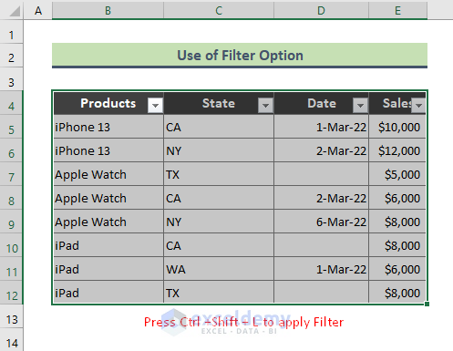
• Let’s filter the 3rd column of the range (B5:E12) based on the Date. Click on the drop-down icon from the Date column, put a checkmark on the Blanks option, and press OK.

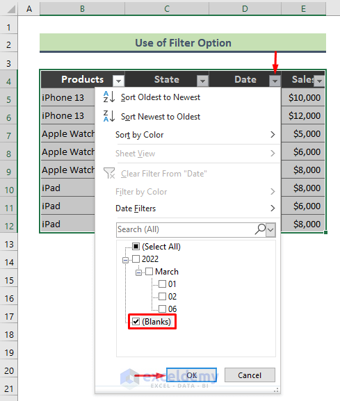
• All the rows that contain the blank cells will be filtered.
• Select all the rows, right-click on the selection, and click Delete Row.

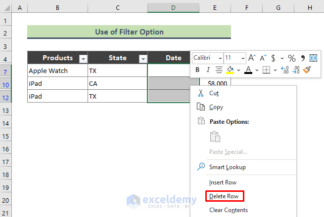
• A message box will ask for the confirmation of row deletion. Click OK.

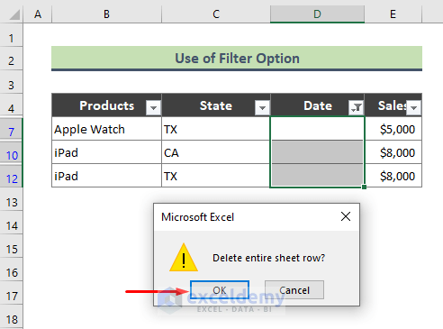
• Withdraw the filter by pressing Ctrl + Shift + L again.

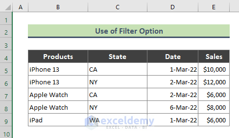
Method 3 – Apply Advanced Filter Feature to Remove Blank Cells from a Range

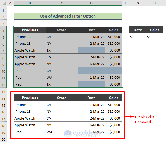
We want to delete the blank cells from two columns (Date and Sales) from our existing dataset.

Steps:

• Put the Date and Sales headers in G4 and H4.
• Put the not equal to (<>) symbol in Cell G5 and H5.

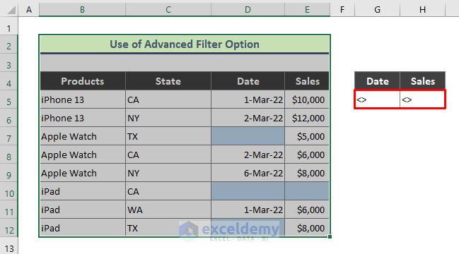
• Go to Data and select Advanced in the Filter group.

• The Advanced Filter dialog shows up.
• Choose Copy to another location, specify List range (B4:E12), Criteria range (G4:H5), Copy to (B4).
• Press OK.

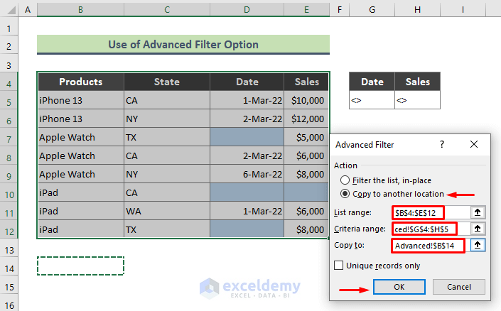
• The range is filtered to another location as below (with blank cells omitted).

⏩ Note:

• The headers of the Criteria range (G4:H5) have to match the parent dataset (B4:E12).

Method 4 – Remove Blank Cells from a Vertical Range

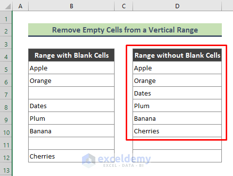
We will use a combination of IFERROR, INDEX, SMALL, IF, MIN, ISBLANK, and ROW functions to delete blank cells present in a vertical range containing fruit names.

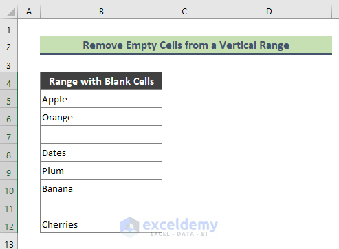
Steps:

• Type the following formula in Cell D5 and hit Enter.

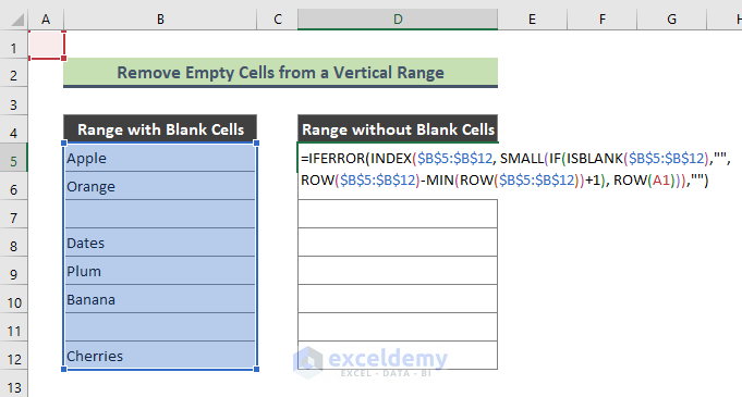
• Drag down the Fill Handle (+) tool to get the result.

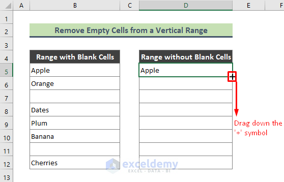
• Blank cells are excluded from the resulting range.

How Does the Formula Work?

• ISBLANK($B$5:$B$12)

Here the ISBLANK function checks whether a cell is blank or not in the range B5:E12 and returns True or False.

• ROW($B$5:$B$12)

{5;6;7;8;9;10;11;12}

• MIN(ROW($B$5:$B$12))

The MIN function finds the lowest row number in the range which is:

{5}

• IF(ISBLANK($B$5:$B$12),””,ROW($B$5:$B$12)-MIN(ROW($B$5:$B$12))+1)

The above formula returns:

{1;2;””;4;5;6;””;8}

• SMALL(IF(ISBLANK($B$5:$B$12),””,ROW($B$5:$B$12)-MIN(ROW($B$5:$B$12))+1), ROW(A1))

Here, the SMALL function returns the k -th smallest value from the range and the formula replies:

{1}

• INDEX($B$5:$B$12,SMALL(IF(ISBLANK($B$5:$B$12),””,ROW($B$5:$B$12)-MIN(ROW($B$5:$B$12))+1), ROW(A1)))

The INDEX formula returns

{“Apple”}

Finally,

• IFERROR(INDEX($B$5:$B$12,SMALL(IF(ISBLANK($B$5:$B$12),””,ROW($B$5:$B$12)-MIN(ROW($B$5:$B$12))+1), ROW(A1))),””)

The IFERROR function returns a blank if the INDEX formula returns an error.

Method 5 – Removing Blank Cells from a Horizontal Range List

We will remove empty cells from a horizontal range of data.

Steps:

• Use the following formula in Cell B8.

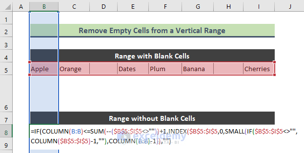
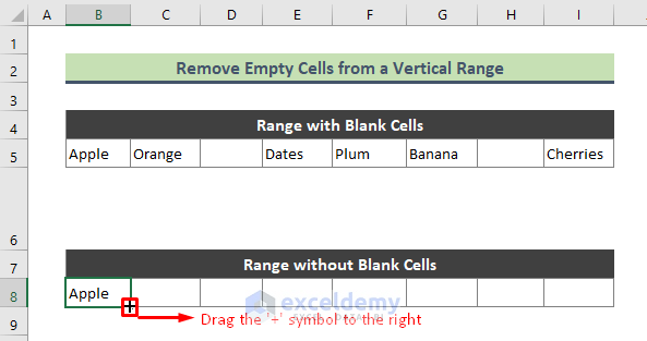
• Once you hit Enter, the formula will give the first non-blank result.
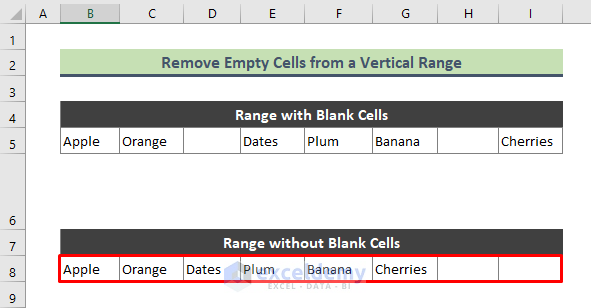
• Drag the Fill Handle tool to the right to get the final output.

• All the blank cells are deleted from the above range.

How Does the Formula Work?

• COLUMN(B:B)<=SUM(–($B$5:$I$5<>””))+1

The above formula returns

{TRUE}

Where,

• COLUMN(B:B)

The COLUMN function replies to column number of B:B which is:

{2}.

• $B$5:$I$5<>””

This will return:

{TRUE,TRUE,FALSE,TRUE,TRUE,TRUE,FALSE,TRUE}

• SUM(–($B$5:$I$5<>””)

The SUM function sums up the count of TRUE values and replies:

{6}

• INDEX($B$5:$I$5,0,SMALL(IF($B$5:$I$5<>””,COLUMN($B$5:$I$5)-1,””),COLUMN(B:B)-1))

The above formula returns:

{“Apple”}

• IF($B$5:$I$5<>””,COLUMN($B$5:$I$5)-1,””)

Here, the IF function checks whether $B$5:$I$5<>””, and returns:

{1,2,””,4,5,6,””,8},

• SMALL(IF($B$5:$I$5<>””,COLUMN($B$5:$I$5)-1,””),COLUMN(B:B)-1)

Later, the SMALL function returns the k-th smallest value from our data range which is:

{1}

• IF(COLUMN(B:B)<=SUM(–($B$5:$I$5<>””))+1,INDEX($B$5:$I$5,0,SMALL(IF($B$5:$I$5<>””,COLUMN($B$5:$I$5)-1,””),COLUMN(B:B)-1)),””)

The above formula returns:

{Apple}

Method 6 – Excel FILTER Function to Delete Empty Cells

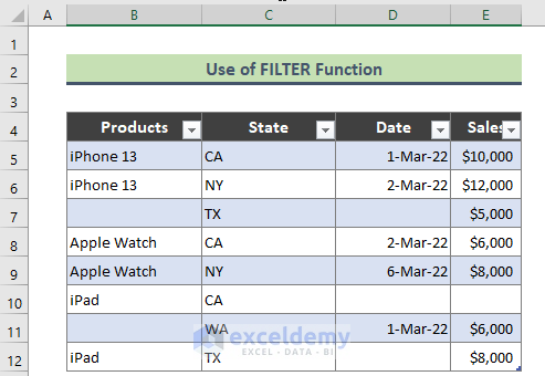
If you are working in Excel 365, you can use the FILTER function to remove blank cells from an Excel range. We will convert the data range (B4:E12) to an Excel table by pressing Ctrl + T.

Steps:

• Use the below formula in Cell B15.

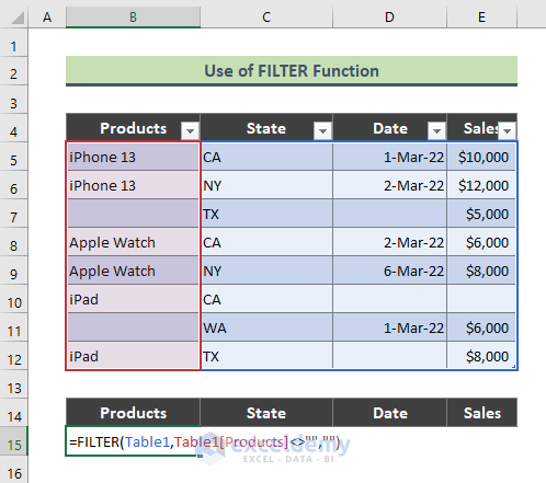
• Press Enter.
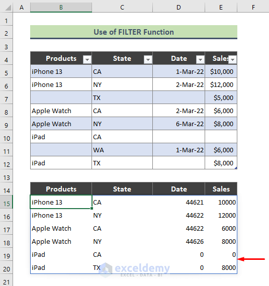
• The above formula will result in an array (outlined in blue color) deleting blank cells from the first column (Products) of the above table.

Read More: How to Remove Blank Cells in Excel

Method 7 – Use the Find Option to Remove Empty Cells from a Range in Excel

Steps:

• Select the range (B5:E12) of data.
• Press Ctrl + F to bring the Find and Replace dialog.
• Leave the Find what field blank, choose Values from the Look in the drop-down, put a checkmark on Match entire cell contents, and press Find All.

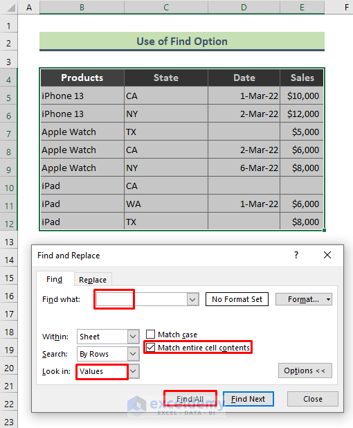
• You will get a list containing the blank cells. Select the whole output by holding the Ctrl key.
• Go to Home then to Cells, pick Delete and choose Delete Cells to bring the Delete dialog.

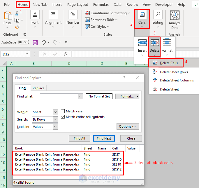
• Choose the delete option and press OK (see screenshot).

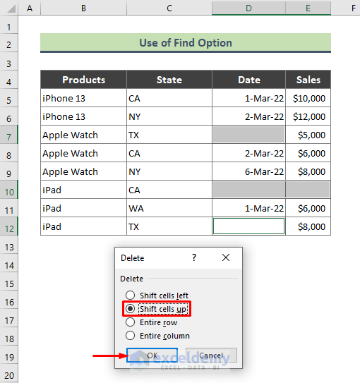
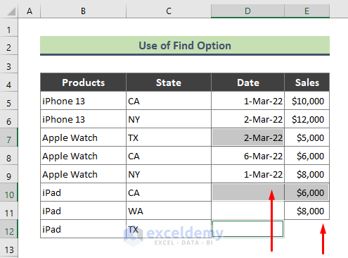
• Here is the output we have received as we have chosen the Shift cells up delete option.
• Click on OK.

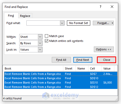
• Press Close to end the process.

Method 8 – Remove Blank Cells from a Range Using the Sort Option

Steps:

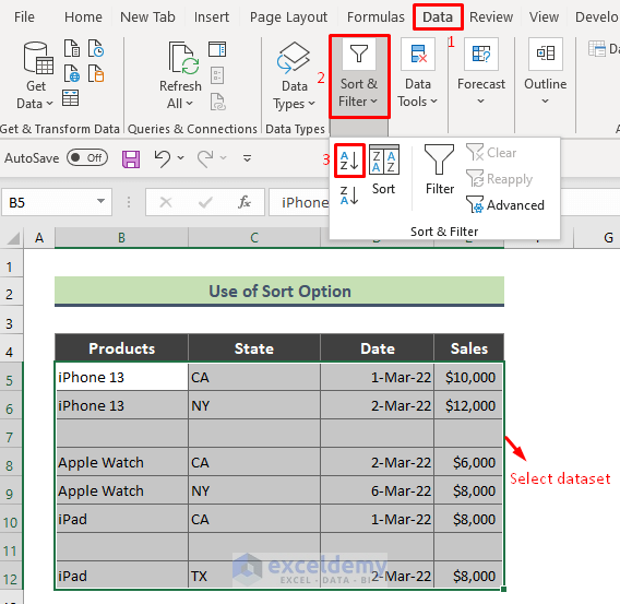
• Select the range.
• Go to Data, choose Sort & Filter, and press the Sort A to Z icon (see screenshot).

• The data range will be sorted. All the blank rows are listed at the end of the range.

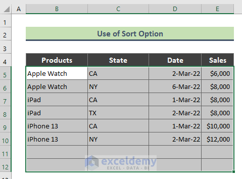
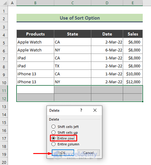
• Press Ctrl + – from the keyboard to bring the Delete dialog.
• Choose the Delete Row option and press OK.

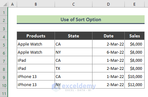
• All the blank rows are deleted from our data range.

Method 9 – Excel Power Query to Delete Empty Cells

We have converted the data range to a table by pressing Ctrl +T.

Steps:

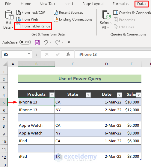
• Click anywhere in the table.
• Go to Data and choose From Table/Range.

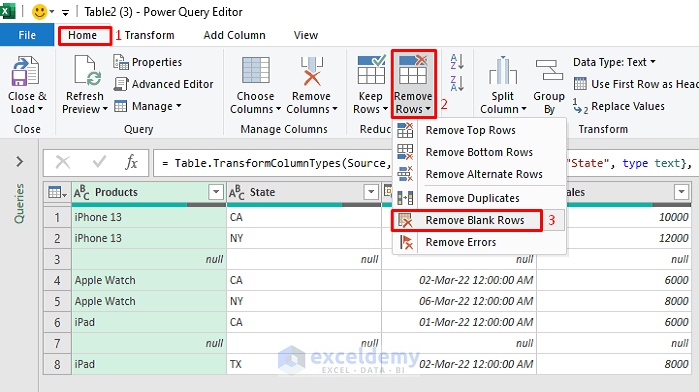
• The table below will show up in the Power Query Editor window.
• By default, null is put in all blank cells.
• Go to Home, choose Remove Rows, and select Remove Blank Rows.

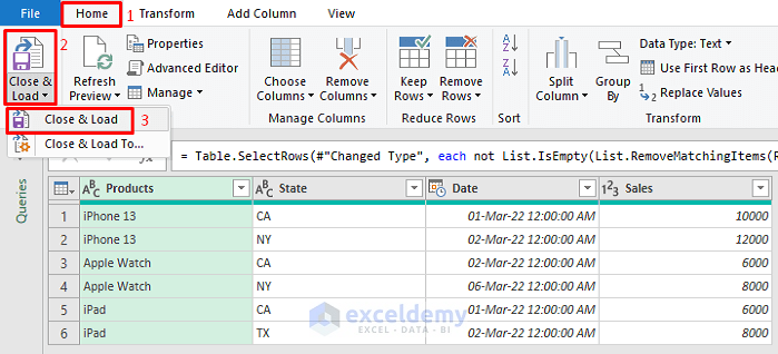
• All the rows that were containing null are removed.
• Go to Home, choose Close & Load, and pick Close & Load.

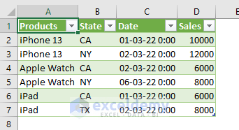
• You’ll get a new table in a new sheet.

Read More: How to Remove Unused Cells in Excel

Download the Practice Workbook

Related Articles

• How to Remove Blank Lines in Excel
• How to Ignore Blank Cells in Range in Excel
• How to Leave Cell Blank If There Is No Data in Excel
• How to Delete Blank Cells and Shift Data Left in Excel

<< Go Back to Blank Cells | Excel Cells | Learn Excel