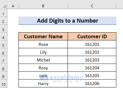
The sample dataset contains 2 columns, Customer Name and Customer ID.
Method 1 – Using the Ampersand(&) Operator to Add Digits to a Number in Excel
1.1. Adding Digits in Front of a Number in Excel
Steps:
- Select a cell to keep the changes. Here, D5.
- Enter this formula.
="10"&C5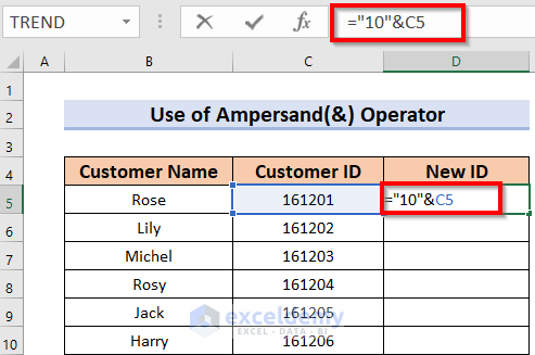
Formula Breakdown
- In the formula, “10”will be added to the number, using the Ampersand (&) operator.
- Press ENTER to see the result.
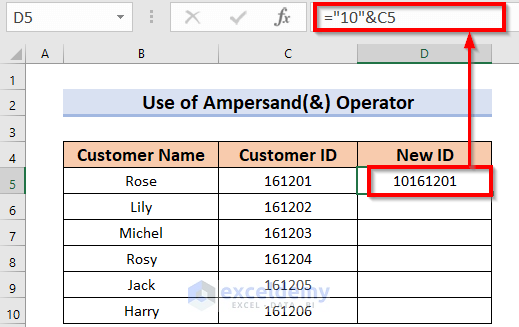
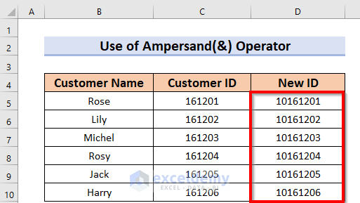
- Drag the Fill Handle to AutoFill the rest of the cells D6:D10.
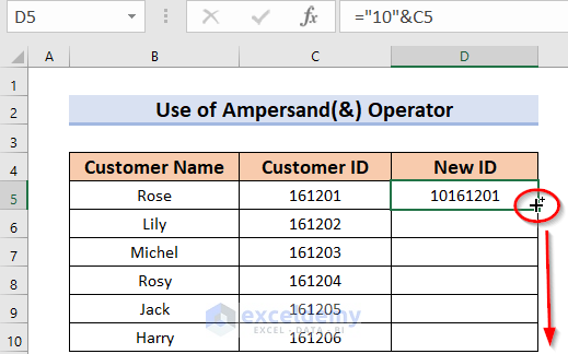
This is the output.
1.2. Adding Digits at the End of a Number in Excel
Steps:
- Select a cell to keep the changes. Here, D5.
- Enter this formula.
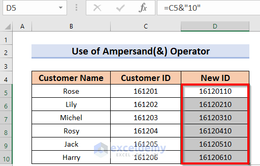
=C5&"10"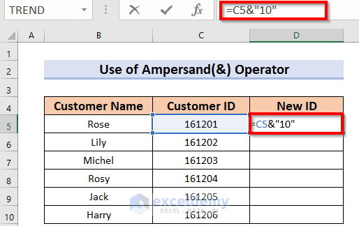
Formula Breakdown
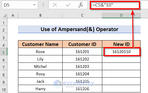
- In the formula, “10”will be added to the number, using the Ampersand (&) operator.
- Press ENTER to see the result.
- Double-click the Fill Handle to AutoFill the range D6:D10.
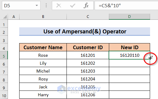
This is the output.
Read More: How to Add Number to Existing Cell Value in Excel
Method 2 – Using the CONCATENATE Function
Steps:
Digits will be added at the end of the number.
- Select a result cell such as D5.
- Enter this formula.
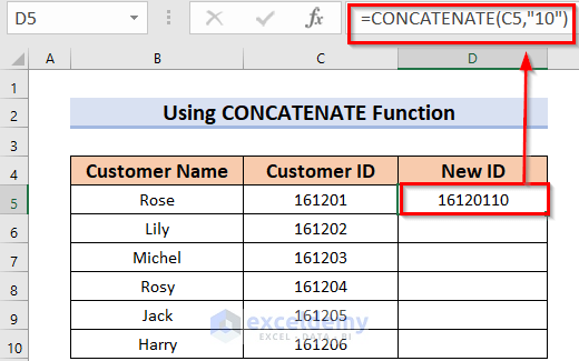
=CONCATENATE(C5,"10")- Press ENTER to see the result.
Formula Breakdown
- The CONCATENATE function will join several texts into one.
- The Inverted Comma (“10”) declares 10 as the string.
- So, CONCATENATE will join 161201 and 10.
- Output: 16120110
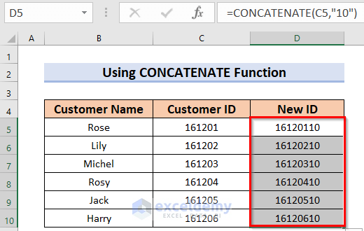
- Double-click the Fill Handle to AutoFill the range D6:D10.
This is the output.
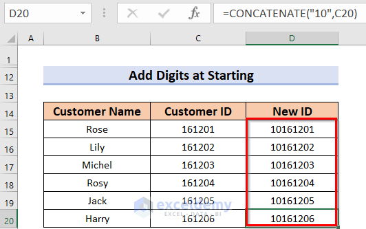
You can also add digits by using the CONCATENATE function.
- Select D15.
- Enter this formula.
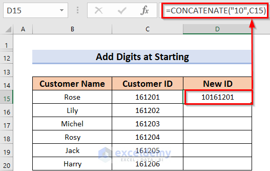
=CONCATENATE("10",C15)- Press ENTER to see the result.
Formula Breakdown
- The CONCATENATE function will join all text to one.
- The Inverted Comma (“10”) declares 10 as a string.
- So, CONCATENATE will join 10 and 161201.
- Output: 10161201
- Drag the Fill Handle to AutoFill the range D16:D20.
Digits were added in front of the number.
Method 3 – Applying the NUMBERVALUE Function and the Ampersand(&) Operator
Steps:
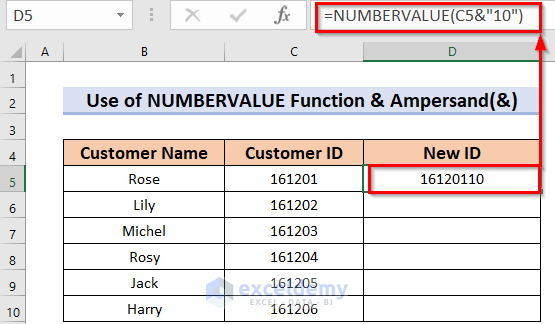
- Select the result cell D5.
- Enter this formula.
=NUMBERVALUE(C5&"10")
- Press ENTER to see the result.
Formula Breakdown
- The NUMBERVALUE function will convert any text to a number format.
- C5 will be the text.
- The Inverted Comma (“10”) declares 10 is a string.
- The Ampersand (&) will join 161201 and 10.
- NUMBERVALUE will convert those strings to the number.
- Output: 16120110
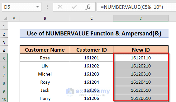
- Double-click the Fill Handle to AutoFill the range D6:D10.
This is the output.
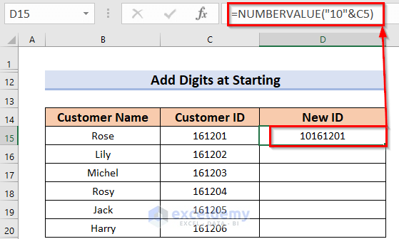
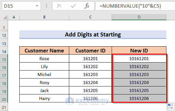
You can also add digits in front of a number in Excel by using the NUMBERVALUE function.
- Select the result cell D5.
- Enter this formula.
=NUMBERVALUE("10"&C5)- Press ENTER to see the result.
Formula Breakdown
- The NUMBERVALUE function will convert text to a number format.
- The Inverted Comma (“10”) declares that 10 is a string.
- Ampersand (&) will join 161201 and 10.
- NUMBERVALUE will convert those strings to the number.
- Output: 10161201
- Double-click the Fill Handle to AutoFill the range D16:D20.
Method 4 – Using the Format Cells Command to Add Digits to a Number in Excel
Add digits to the end of a number.
Steps:
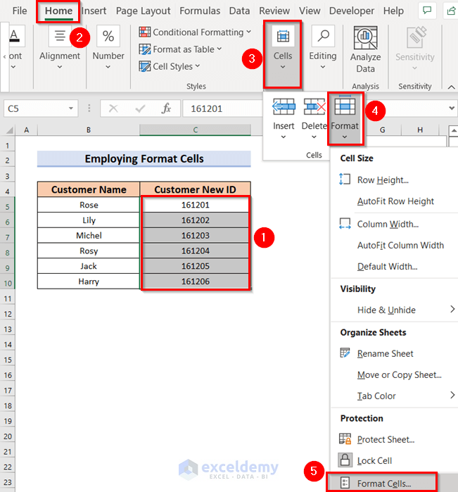
- Select the data range. Here, C5:C10.
- In the Home tab >> go to Cells.
- In Format >> choose the Format Cells command.
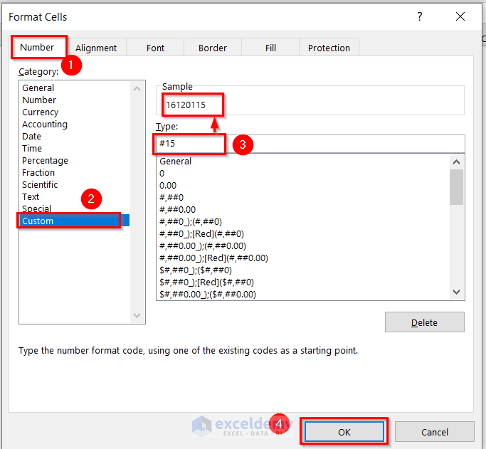
In the Format Cells dialog box:
- Choose the Number command.
- Select Custom.
- Enter your digits with a Hashtag (#) at the beginning. We used #15.
- Click OK to see the result.
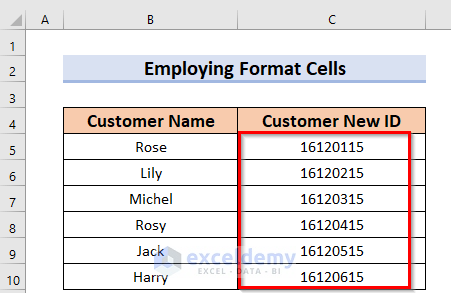
This is the output.
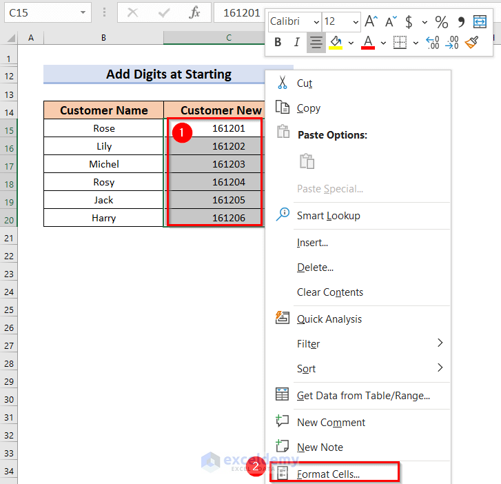
To add digits in front of a number.
- Select the data range. Here, C15:C20.
- Right-Click the data.
- In the Context Menu Bar, choose Format Cells.
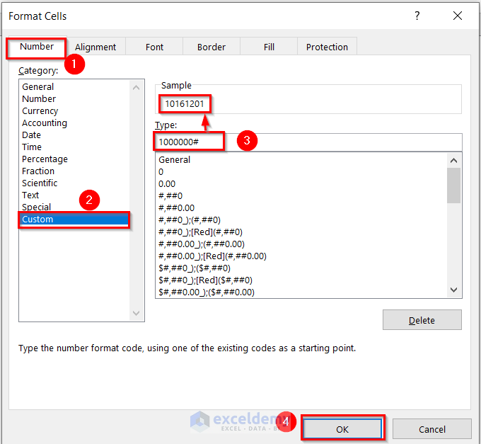
In the Format Cells dialog box:
- Choose the Number command.
- Select Custom.
- Enter your digits with a Hashtag (#) at the end. Here, 1000000#. If you want to add a zero (0), you must enter 6 zeroes. 5 zeroes is a constant to include 1 zero.
- Press OK to see the result.
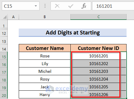
This is the output.
Method 5 – Using the Format Cells Feature to Add Digits in the Middle of a Number
Steps:
- Select the data range. Here, C5:C10.
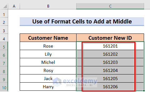
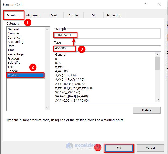
- Press CTRL+1 to open the Format Cells dialog box.
In the Format Cells dialog box:
- Choose the Number command.
- Select Custom.
- Enter your digits with a Hashtag (#) at the beginning. Include the zeroes. Zero is the position of the written digits at the end of the number. Here, #55000. 55 will be in the 4th position of the rightmost part.
- Click OK to see the result.
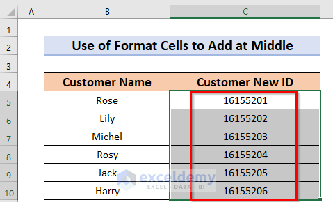
This is the output.
Method 6 – Using the LEFT Function and the Ampersand(&) Operator
Steps:
Digits will be added at the end of a number.
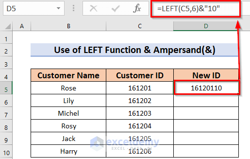
- Select a cell, in which you want to keep the changes. Here, D5.
- Enter this formula.
=LEFT(C5,6)&"10"- Press ENTER to see the result.
Formula Breakdown
- LEFT(C5,6)—->The LEFT function will count the leftmost 6 characters in C5.
- Output: 161201
- “10”—-> Inverted Comma will declare 10 as a string.
- & —-> Ampersand (&) will join 161201 and 10.
-
- Output: 16120110
- Double-click the Fill Handle to AutoFill the rest of the cells: D6:D10.
This is the output.
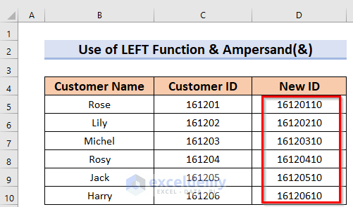
You can also add digits in front of a number in Excel by using the LEFT function.
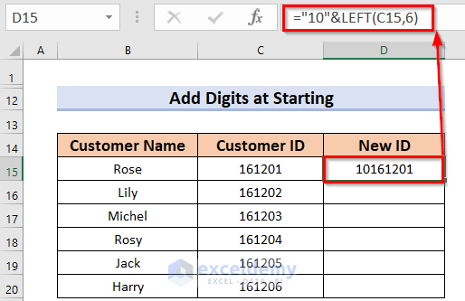
- Select a cell, to keep the changes. Here, D15.
- Enter this formula.
="10"&LEFT(C15,6)- Press ENTER to see the result.
Formula Breakdown
- “10”—-> Inverted Comma declares 10 as a string.
- LEFT(C15,6)—->Here, the LEFT function will count the leftmost 6 characters in C15.
- Output: 161201
- & —-> Ampersand (&) will join 10 and 161201.
-
- Output: 10161201
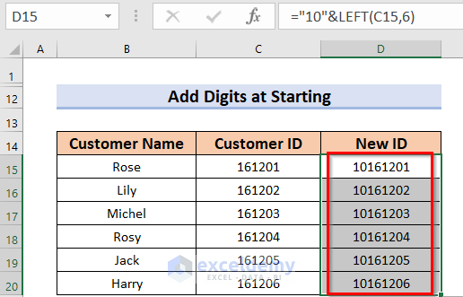
- Drag the Fill Handle to AutoFill the rest of the cells: D16:D20.
This is the output.
Method 7 – Using the MID Function and the Ampersand(&) Operator
Steps:
Digits will be added at the end of the number.
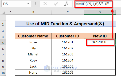
- Select a cell to keep the changes. We used D15.
- Enter this formula.
=MID(C5,1,6)&"10"- Press ENTER to see the result.
Formula Breakdown
- MID(C5,1,6)—-> The MID function will extract 6 characters starting from the 1st character in C5.
- Output: 1612010
- “10”—-> Inverted Comma declares 10 as a string.
- & —-> Ampersand (&) will join 161201 and 10.
- Output: 16120110
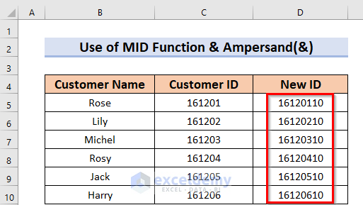
- Drag the Fill Handle to AutoFill the rest of the cells: D6:D10.
You can also add digits in front of the number in Excel using the MID function.
- Select the result cell D15.
- Enter this formula.
="10"&MID(C15,1,6)- Press ENTER to see the result.
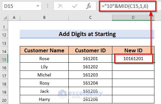
Formula Breakdown
- “10”—-> Inverted Comma declares 10 as a string.
- MID(C15,1,6)—-> The MID function will extract 6 characters starting from the 1st character in the cell C15.
- Output: 1612010
- & —-> Ampersand (&) will join 10 and 161201.
- Output: 10161201
- Drag the Fill Handle to AutoFill the rest of the cells: D16:D20.
This is the output.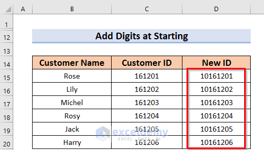
Method 8 – Applying the LEFT and MID Functions with the Ampersand(&) Operator
Steps:
- Select a cell to keep the changes. Here, D5.
- Enter this formula.
=LEFT(C5,3)&"55"&MID(C5,4,3)- Press ENTER to see the result.
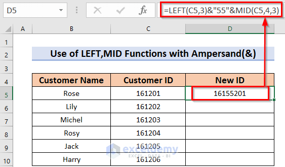
Formula Breakdown
- LEFT(C5,3)—->The LEFT function will count the leftmost 3 characters in C5.
- Output: 161
- “55”—-> Inverted Comma declares 55 as a string.
- MID(C5,4,3)—-> The MID function will extract 3 characters starting from the 4th character in C5.
- Output: 201
- & —-> Ampersand (&) will join 161, 55, and 201.
-
- Output: 16155201
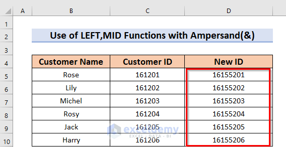
- Drag the Fill Handle to AutoFill the rest of the cells: D6:D10.
This is the output.
Practice Section
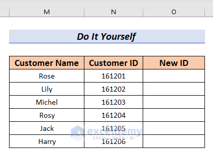
Use the following dataset to test these methods.
Download the Practice Workbook
Related Articles
<< Go Back to Add to Cell Value | Sum in Excel | Calculate in Excel | Learn Excel
Get FREE Advanced Excel Exercises with Solutions!

