Advanced Conditional Formatting with Formula-Based Rules

Conditional formatting is a powerful Excel feature that automatically applies formatting like colors, icons, or bold fonts based on the values of the spreadsheet. Though Excel offers easy-to-use built-in rules for conditional formatting, formula-based rules provide greater flexibility. In this tutorial, we will show advanced conditional formatting using formula-based rules, which gives you far greater flexibility than standard built-in options.

Creating a Formula-Based Conditional Formatting Rule

Conditional Formatting works based on certain conditions, and it also offers formula-based customized rules. Formula-based conditional formatting defines rules using custom formulas that evaluate the data in your worksheet. The formatting is applied when the formula returns TRUE. To apply the formula-based rule you will need to follow certain steps:

• Select the cell range to apply conditional formatting.
• Go to the Home tab >> from Conditional Formatting >> select New Rule.
• In the New Formatting Rule dialog box;
  • Select the option Use a formula to determine which cells to format.
  • In the Format values where this formula is true box;
    • Insert the custom formula.
  • Click on Format to select the format of your choice.
  • Click OK.

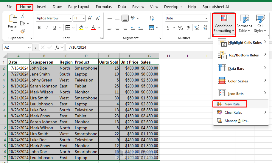
Let’s consider a sales dataset to apply advanced conditional formatting with formula-based rules.

1. Highlight Rows Based on a Condition

If you want to highlight rows where sales are greater than a certain value, you can use the following comparison formula.

Formula:

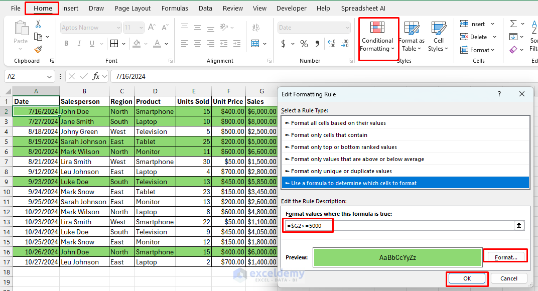
=$G2>=5000

This formula checks if the value in cell C2 (Sales) is greater than 5000. Use absolute reference ($) for columns if the comparison is consistent across the rows.

• Click Format and set your preferred formatting options, we selected the color green.
• Click OK to apply the rule.

2. Highlight Duplicates Sales Entries

You can highlight duplicate sales entries from your dataset to remove those entries. Insert the following formula.

Formula:

=COUNTIFS($A$2:$A$17, $A2, $B$2:$B$17, $B2, $C$2:$C$17, $C2, $D$2:$D$17, $D2, $E$2:$E$17, $E2, $F$2:$F$17, $F2, $G$2:$G$17, $G2) > 1

This formula checks each column from A to G to determine if the combination of values in each row is duplicated within the specified range, then it counts each row’s unique combination of values in columns A to G. If the count is greater than 1, the row is considered duplicate. Then the row is highlighted as duplicates.

• Click Format, and choose your formatting, we selected yellow fill.
• Click OK to apply the rule.

3. Color Every Other Row (Zebra Striping)

To format the data table and make it easy to read you can add color to every other row. To add this format, use the following formula.

Formula:

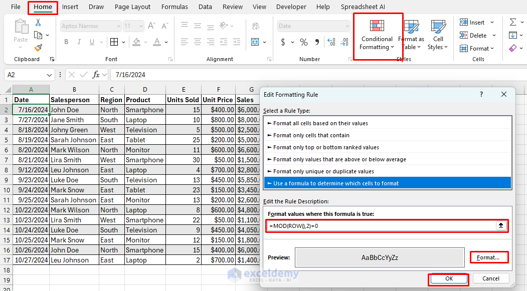
=MOD(ROW(),2)=0

The ROW() function returns the current row number. Then the MOD(ROW(),2)=0 checks if the row number is even.

• Click Format, and choose your formatting, we selected light gray background fill.
• Click OK to apply the rule.

4. Highlight Past Dates

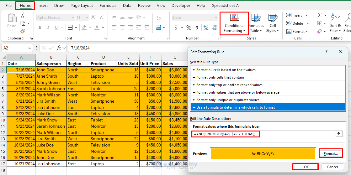
If you want to highlight dates that are past today’s date to identify overdue items, you can do it by using the formula of the TODAY function.

Formula:

=AND(ISNUMBER(A2), A2 < TODAY())

This formula checks if the date in A2 is before today’s date to highlight any past dates in your dataset.

• Click Format, and choose your formatting, we selected red fill.
• Click OK to apply the rule.

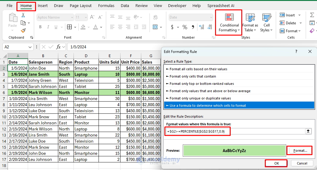
5. Highlight Top 10% Sales Values

You can highlight the top 10% of sales of your sales dataset. To highlight the top sales, you can use the PERCENTILE function.

Formula:

=$G2>=PERCENTILE($G$2:$G$17,0.9)

The PERCENTILE($G$2:$G$17,0.9) calculates the 90th percentile of the range, so values greater than or equal to this are in the top 10%. If a value in column G is greater than or equal to this percentile, the formatting will be applied to the entire row.

• Click Format, and choose your formatting, we selected bold text with a green fill color.
• Click OK to apply the rule.

6. Combining Multiple Conditions

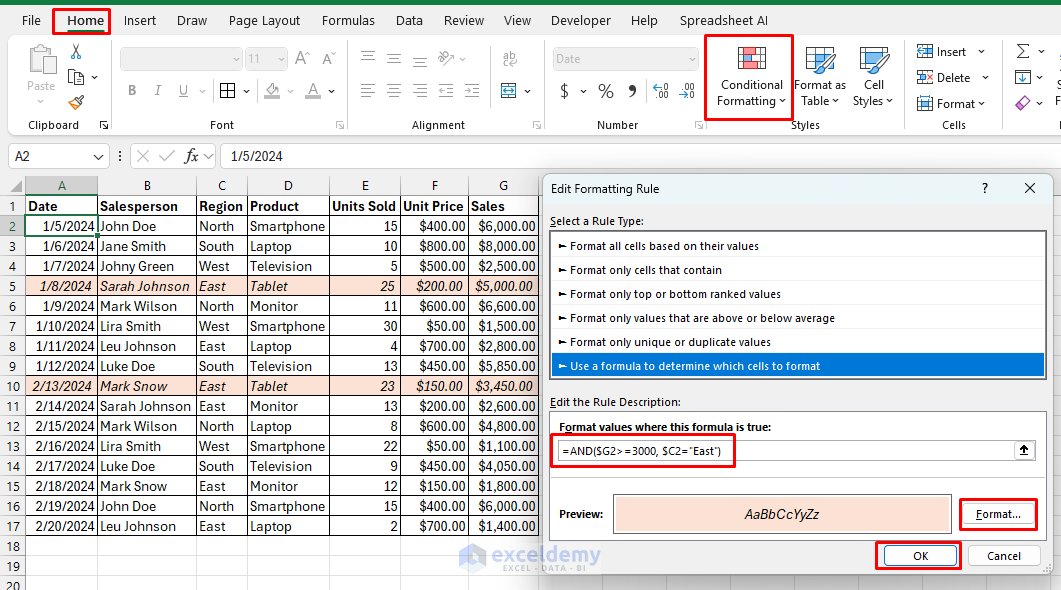
You can create complex conditional formatting rules by combining multiple conditions with logical functions. Using AND/OR functions to Highlight cells based on multiple conditions.

Formula:

=AND($G2>=3000, $C2=”East”)

This formula highlights the rows only if sales are greater than or equal to 3000 and the region is east.

• Click Format, and choose your formatting, we selected italic font and peach fill color.
• Click OK to apply the rule.

Managing Conditional Formatting Rules

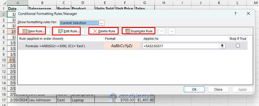
To manage your conditional formatting:

• Go to the Conditional Formatting tab >> select Manage Rules.
• Here you can view, add, edit, delete, duplicate, or change the priority of your rules.
• You can also use the “Applies to” field to modify the cell range to apply the rules.

Conclusion

You can use advanced conditional formatting with formula-based rules in Excel to highlight your data. It gives a flexible way to visualize data. Whether you’re highlighting cells based on specific conditions, managing duplicates, combining multiple criteria, or checking due dates these formula-based rules will help you. Mastering this feature will make your spreadsheets more insightful and visually appealing. Experiment with different formulas to see how they work and enhance your spreadsheets.