Method 1 – Using a Nested IF Formula
We’ll work with a dataset containing names and ages. Our goal is to determine the appropriate team for each person based on their age.
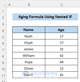
- Select cell D5.
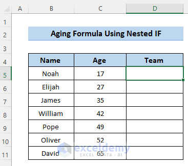
- Enter the following formula in the formula box:
=IF(C5<20,"Avengers",IF(C5<40,"Panthers",IF(C5<60,"Lions","Warriors")))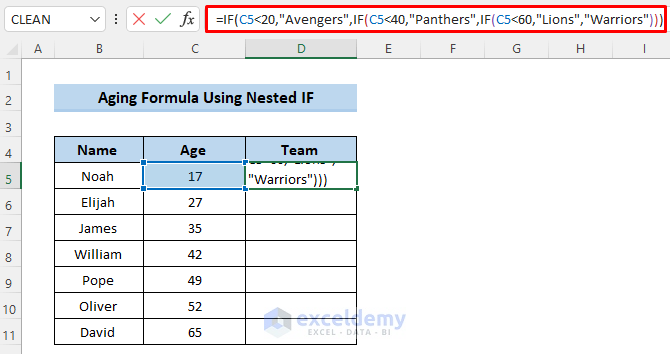
- Press Enter to apply the formula.
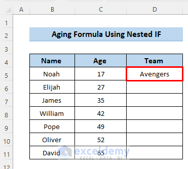
- Drag the Fill handle icon down the column to cell D11.
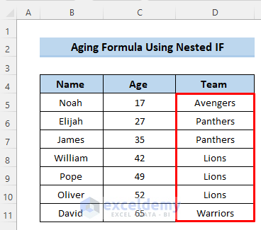
Breakdown of the Formula
IF(C5<20,”Avengers”,IF(C5<40,”Panthers”,IF(C5<60,”Lions”,”Warriors”)))
⇒ IF(C5<20,”Avengers” …): If the value in cell C5 is less than 20 (indicating an age below 20), it will return “Avengers.” Otherwise, it moves to the next condition.
⇒ IF(C5<40,”Panthers” ….): If the value in cell C5 is less than 40 (but not less than 20), it will return “Panthers.” Otherwise, it moves to the next condition.
⇒ When the value of cell C5 doesn’t match the first two conditions, it will automatically move to the third condition.
⇒ IF(C5<60,”Lions” ….): If the value in cell C5 is less than 60 (but not less than 40), it will return “Lions.” Otherwise, it defaults to “Warriors” for ages above 60.
⇒ Finally, if the value of C5 doesn’t meet any of the conditions above, it will automatically return a string “Warriors”. Actually, it means if the age limit of cell C5 is above 60, it will be in the Warriors group.
Method 2 – Aging Formula for Number of Days Worked
We’ll determine the aging bucket for the number of days an employee has worked.
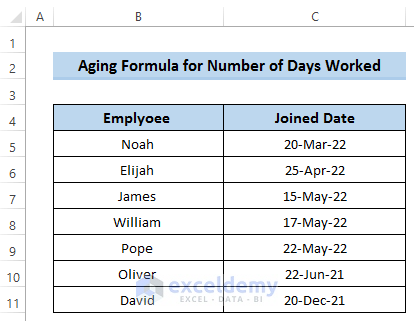
- Select cell D5.
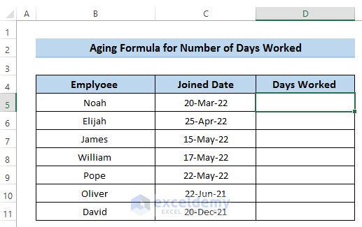
- Enter the following formula in the formula box:
=TODAY()-C5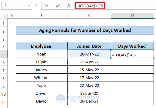
- Press Enter to apply the formula.
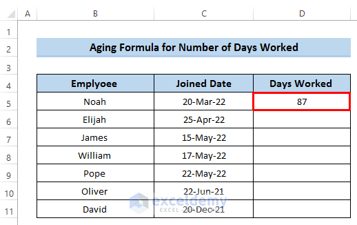
- Drag the Fill handle icon down the column to cell D11.
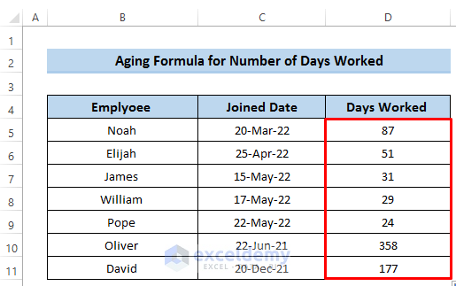
Breakdown of the Formula
TODAY()-C5
This formula calculates the difference between today’s date and the date in cell C5, giving us the number of days worked by the employee.
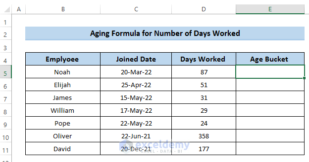
- Select cell E5 and enter the following formula:
=IF(D5<=60,"Less than 2 Months",IF(D5<=120,"2 Months+",IF(D5<=180,"4 Months+","6 Months+")))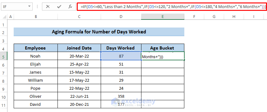
- Press Enter to apply the formula.
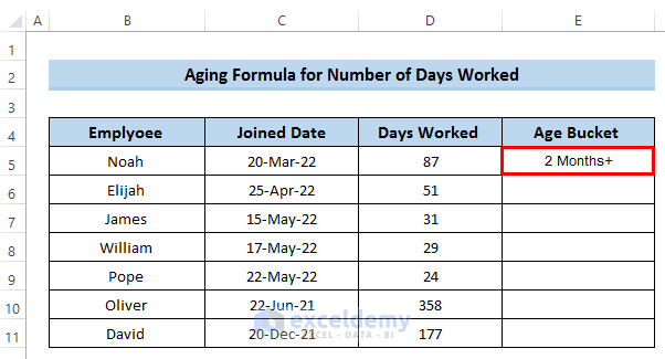
- Drag the Fill handle icon down the column to cell E11.
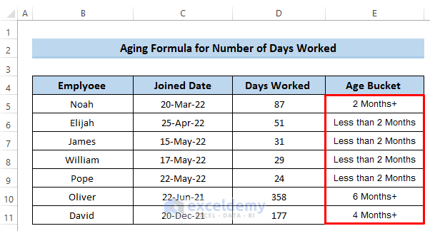
Breakdown of the Formula
IF(D5<=60,”Less than 2 Months”,IF(D5<=120,”2 Months+”,IF(D5<=180,”4 Months+”,”6 Months+”)))
⇒ IF(D5<=60,”Less than 2 Months”….): It demonstrates when the value of cell D5 is less than or equal to 60, it will return the string “Less than 2Months”. That means if the employee worked less than equal to 60 days, it will automatically go to the Less than 2 Months section. If the value of cell D5 doesn’t meet the condition, it will automatically go to the next condition.
⇒ IF(D5<=120,”2 Months+”….): When the cell value doesn’t meet the above condition, it will come to this condition to look up whether it meets this one or not. This formula denotes if the value of cell D5 is less than or equal to 120, it will return the string “2 Months+”. That means if the employee worked less than equal to 120 days, it will automatically go to the 2 Months+ sections. If the value of cell D5 doesn’t meet the condition, it will automatically go to the next condition.
⇒ IF(D5<=180,”4 Months+”….): This formula denotes if the value of cell D5 is less than or equal to 180, it will return a string called “4 Months+”. This actually demonstrates. If it doesn’t meet the condition, it will automatically go to the next condition.
If the value of C5 doesn’t meet any of the conditions above, it will automatically return a string “6 Months+”. Actually, it means if the age limit of cell C5 is above 180, it will be in the 6 Months + group.
Method 3 – Using IF Formula to Determine Expiration Days
We’ll work with product expiration dates to create an age bucket using the IF function.
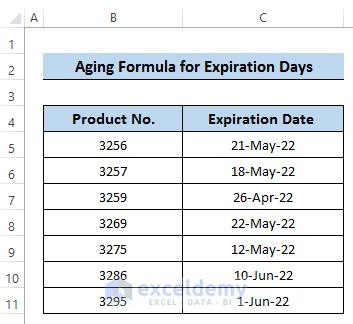
- Select cell D5.
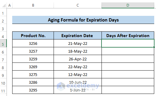
- Enter the following formula in the formula box:
=TODAY()-C5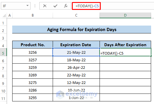
- Press Enter to apply the formula.
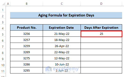
- Drag the Fill handle icon down the column to cell D11.
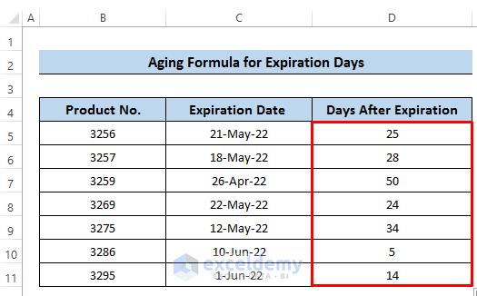
Breakdown of the Formula
TODAY()-C5
This formula calculates the difference between today’s date and the date in cell C5, giving us the number of days after the product’s expiration.
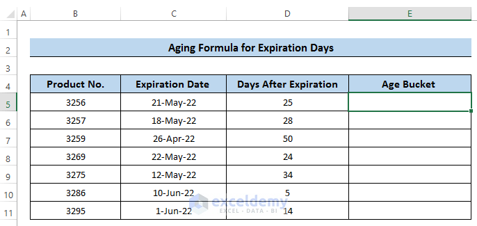
- Select cell E5 and enter the following formula:
=IF(D5<=15,"Less than 15 days",IF(D5<30,"Between 15 and 30 days","More than 30 days"))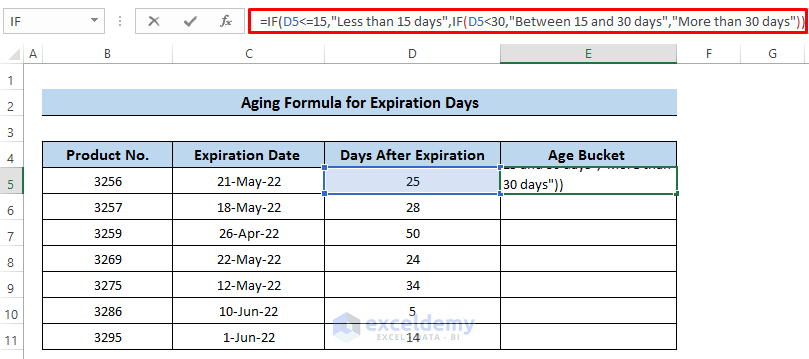
- Press Enter to apply the formula.
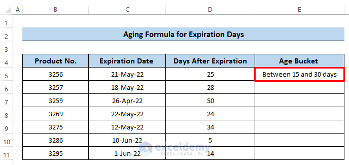
- Drag the Fill handle icon down the column to cell E11.
This formula categorizes the days after expiration into different buckets based on the number of days.
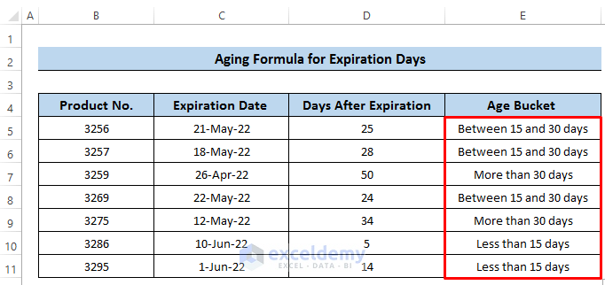
Breakdown of the Formula
IF(D5<=15,”Less than 15 days”,IF(D5<30,”Between 15 and 30 days”,”More than 30 days”))
⇒ IF(D5<=15,”Less than 15 days”….): If the value in cell D5 is less than or equal to 15, it will return “Less than 15 days.” This means that if the product has passed its expiration date by 15 days or less, it falls into this category. If the value of cell D5 doesn’t meet this condition, it moves to the next condition.
⇒ IF(D5<30,”Between 15 and 30 days”….): If the value in cell D5 is less than 30 (but not less than 15), it will return “Between 15 and 30 days.” This category covers products with expiration dates between 15 and 30 days. If the value of cell D5 doesn’t meet this condition, it defaults to “More than 30 days” for products with expiration dates beyond 30 days.
⇒ Finally, if the value of C5 doesn’t meet any of the conditions above, it will automatically return a string “More than 30 days”. Actually, it means if the expiration date of the product is above 30 days, it will be in the More than 30 days group.
Method 4 – Combining IF with AND Function
We’ll create an aging report based on invoice data.
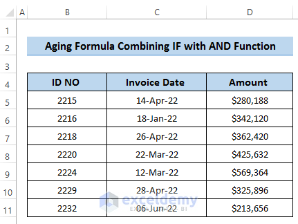
- Select cell E5.
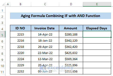
- Enter the following formula to calculate the days past:
=TODAY()-C5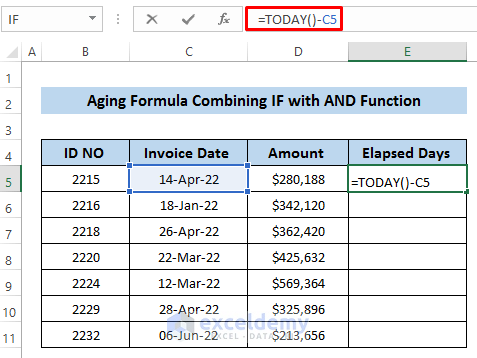
- Press Enter to apply the formula.
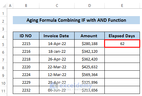
- Drag the Fill Handle icon down the column up to cell E11.
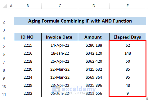
- Invoices Below 30 Days: Select cell F5.
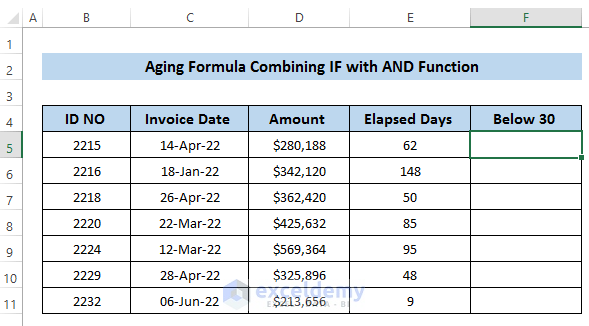
- Enter the following formula:
=IF(E5<=30,D5,0)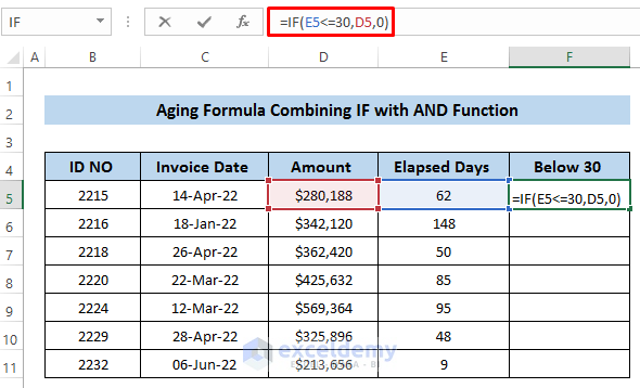
- Press Enter to apply the formula.
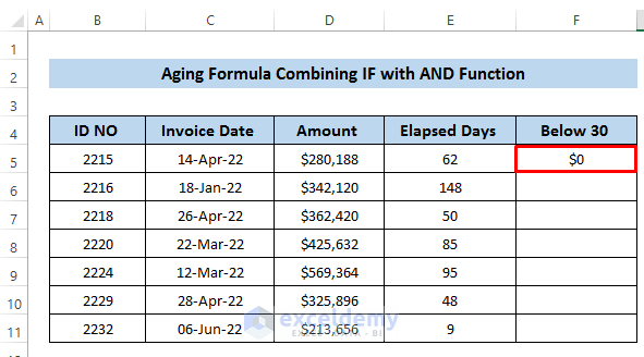
- Drag the Fill handle icon down the column. You’ll see only one invoice amount in this section.
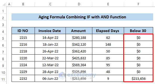
Breakdown of the Formula
IF(E5<=30,D5,0)
If the value in cell E5 is less than or equal to 30, it returns the invoice amount (cell D5); otherwise, it returns 0.
- Invoices Between 31 and 60 Days: Select cell G5.
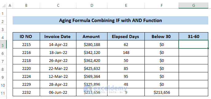
- Enter the following formula:
=IF(AND(E5>30,E5<=60),D5,0)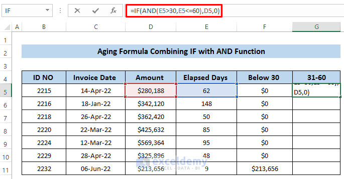
- Press Enter to apply the formula.
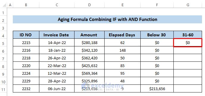
- Drag the Fill handle icon down the column.
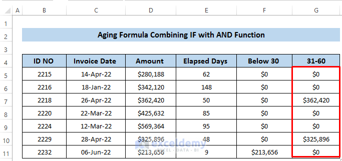
Breakdown of the Formula
IF(AND(E5>30,E5<=60),D5,0)
⇒ AND(E5>30,E5<=60): This condition checks if the value of cell E5 is greater than 30 and less than or equal to 60.
⇒ IF(AND(E5>30,E5<=60),D5,0): If the condition is met, it returns the invoice amount (cell D5); otherwise, it returns 0.
- Invoices Between 61 and 90 Days: Select cell H5.
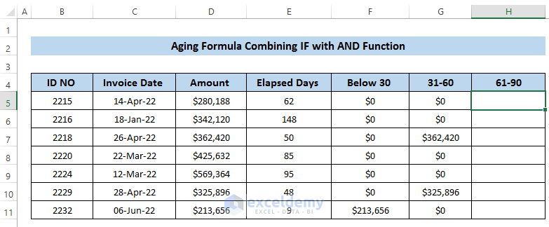
- Enter the following formula:
=IF(AND(E5>60,E5<=90),D5,0)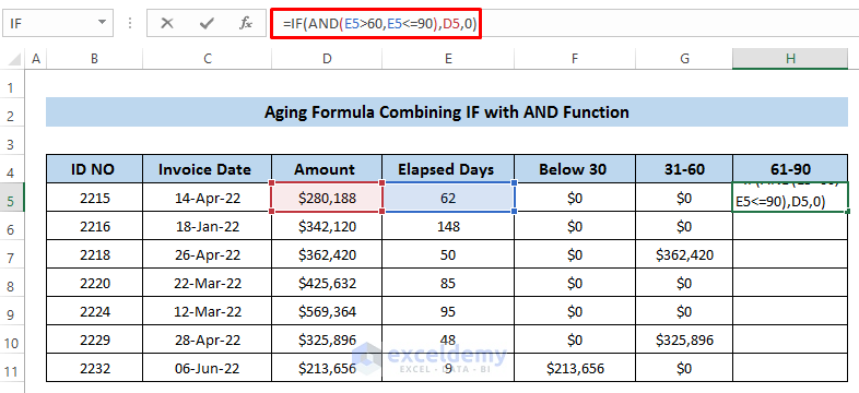
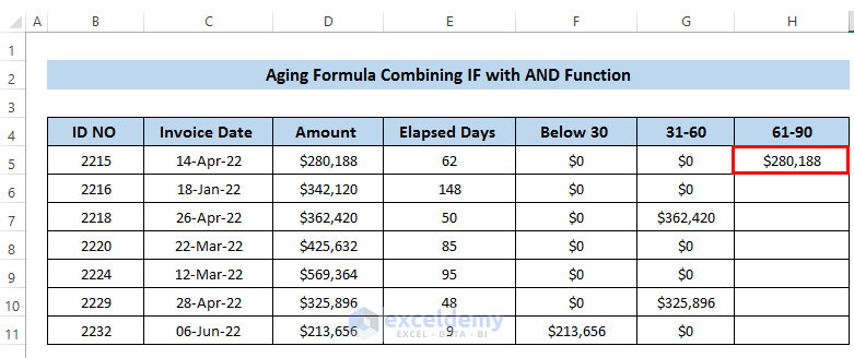
- Press Enter to apply the formula.
- Drag the Fill Handle icon down the column.
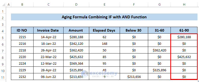
- Invoices Above 90 Days: Select cell I5.
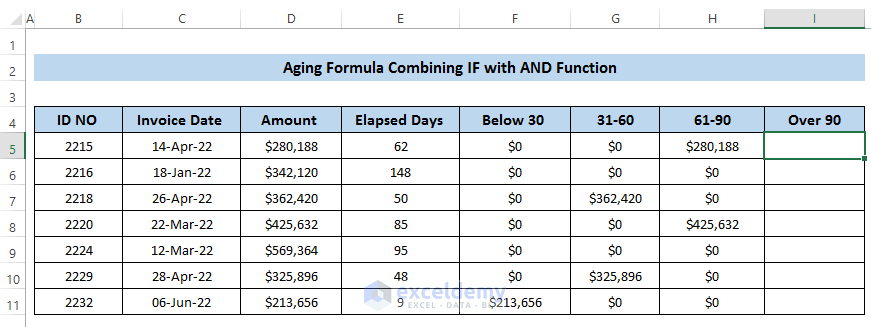
- Enter the following formula:
=IF(E5>90,D5,0)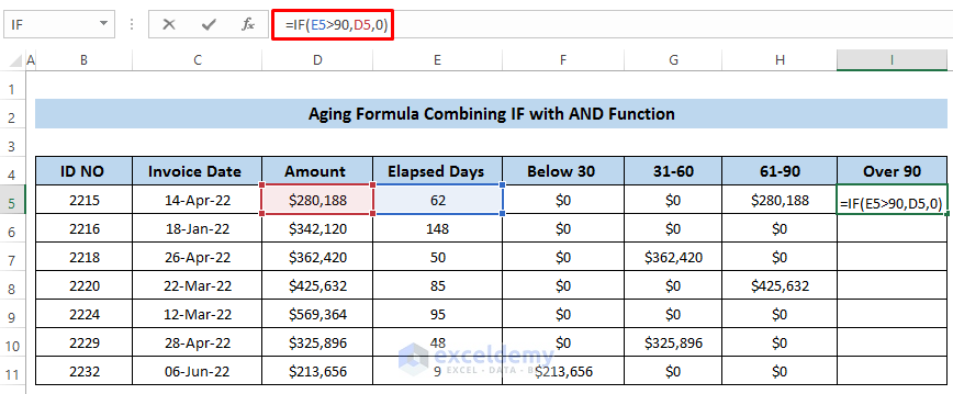
- Press Enter to apply the formula.
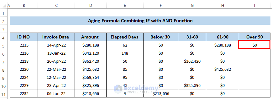
- Drag the Fill Handle icon down the column.
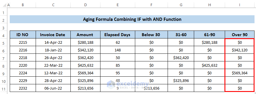
Breakdown of the Formula
IF(E5>90,D5,0)
If the value of cell E5 is greater than 90, it returns the invoice amount (cell D5); otherwise, it returns 0.
Download the Practice Workbook
You can download the practice workbook from here:
<< Go Back to Ageing | Formula List | Learn Excel
Get FREE Advanced Excel Exercises with Solutions!

