In this article, we will demonstrate how to AutoFill sequential letters in Excel (A, B, C, D, etc.). We’ll use the following dataset where a Gate No is associated with a Watchman’s Name, and Autofill the gate numbers sequentially using various methods.
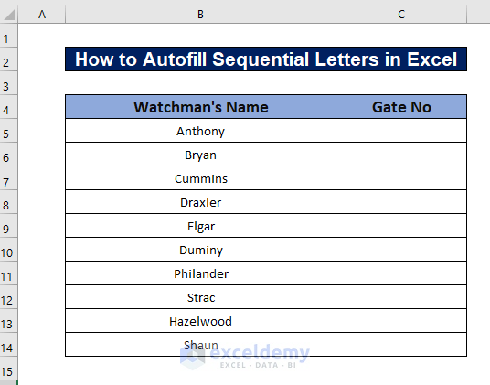
Method 1 – Using CHAR & CODE Functions
The use of the CHAR function and CODE function is one of the easiest ways to AutoFill sequential letters in Excel.
Steps:
- In cell C5, enter the first letter, A.
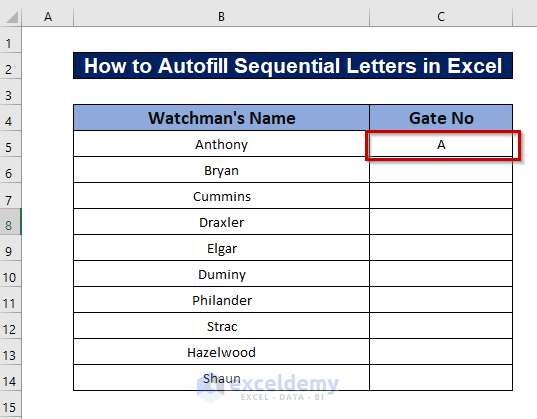
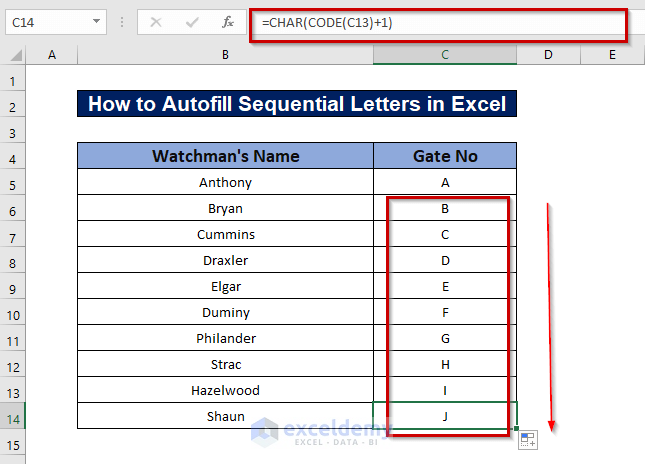
- Input the following formula in cell C6:
=CHAR(CODE(C5)+1)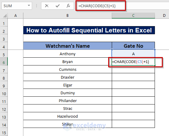
Formula Breakdown
- CODE(C5) —–> returns the character code of the value in cell C5.
- Output: 65
- CHAR(CODE(C5)+1)
- CHAR(65+1) —–> returns the ASCII character of the code + 1.
- Output: “B”
- Press ENTER.
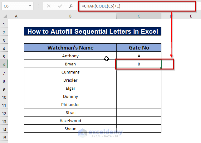
The sequential value of B is returned.
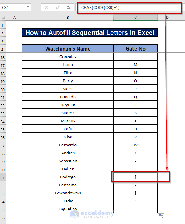
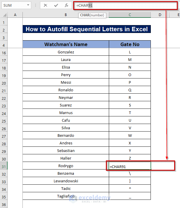
- Drag the Fill Handle down to AutoFill the formula for the rest of the cells.
Read More: [Fixed!] AutoFill Formula Is Not Working in Excel Table
Method 2 – Using SUBSTITUTE Function
We can also use the SUBSTITUTE function along with the ADDRESS and ROW functions.
Steps:
- Enter the following formula in cell C5:
=SUBSTITUTE(ADDRESS(1,ROWS($A$1:$A1),4),1,"")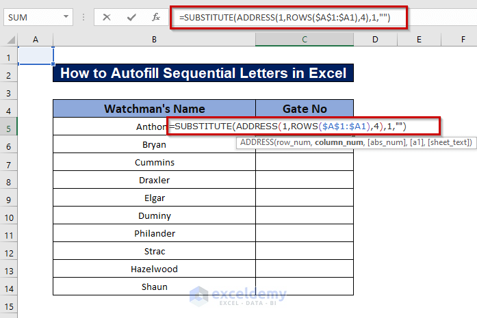
Formula Breakdown
- ROWS($A$1:$A1) —> returns the number of rows in the specified range.
- Output: 1
- ADDRESS(1,1,4) —> returns the address at the specified row_num and col_num.
- Output: “A1”
- SUBSTITUTE(ADDRESS(1,ROWS($A$1:$A1),4),1,” “)
- SUBSTITUTE(‘A1’,1,””) —–> substitutes 1 character from the left side of the text, here a “1” with a blank.
- Output: A
- Press ENTER.
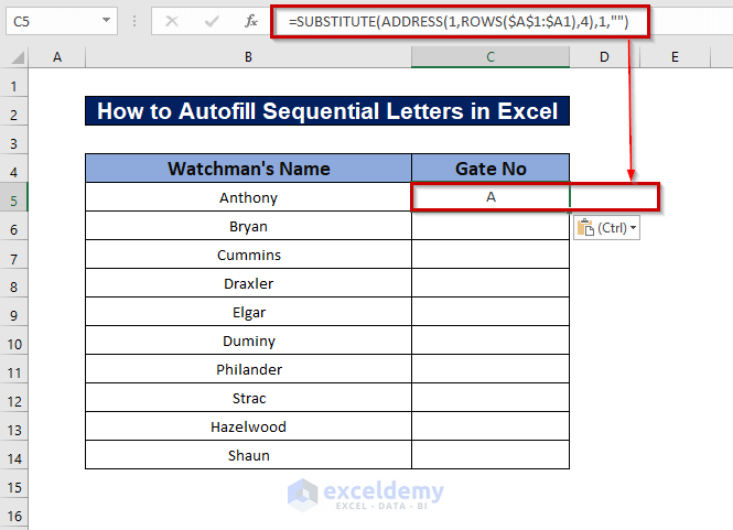
We have the first letter, A.
- Use the Fill Handle to AutoFill the formula for the rest of the cells.
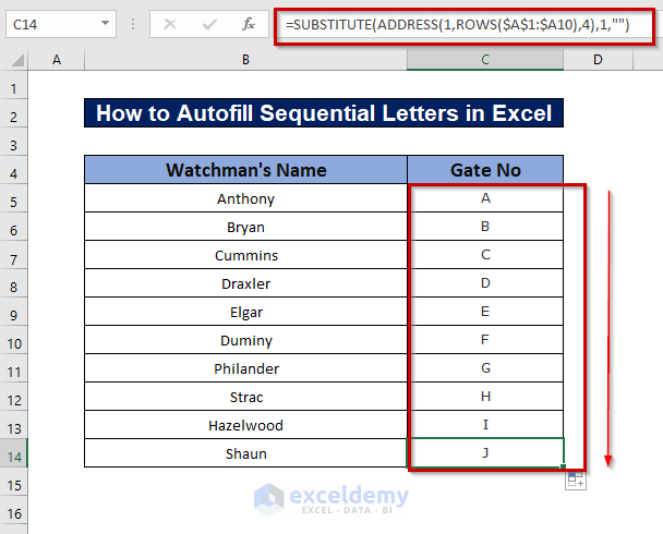
Read More: How to AutoFill from List in Excel
Method 3 – Using LEFT Function
Another efficient method is to use the LEFT function including the ADDRESS function and ROW function.
Steps:
- Enter the following Formula in cell C5:
=LEFT(ADDRESS(1,ROW(A1),4,1),(ROW(A1)>26)+1)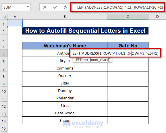
Formula Breakdown
- ROW(A1) —–> returns the row number of the referenced cell.
- Output: 1
- ADDRESS(1,1,4,1) —–> returns the address of the specified row_num and col_num.
- Output: “A1”
- (ROW(A1)>26) —–> checks whether the row number is greater than 26 or not.
- Output: FALSE
- FALSE+1 —–> becomes
- Output: 1
- LEFT(ADDRESS(1,ROW(A1),4,1),(ROW(A1)>26)+1)
- LEFT({“A1”},{1}) —–> extracts 1 character from the left side of the text.
- Output: A
- Press ENTER.
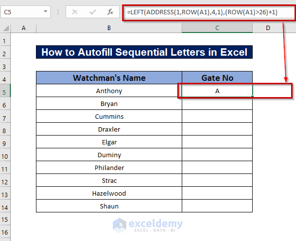
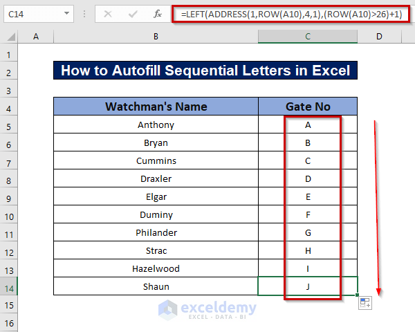
- Use the Fill Handle to AutoFill the formula in a column for the rest of the cells.
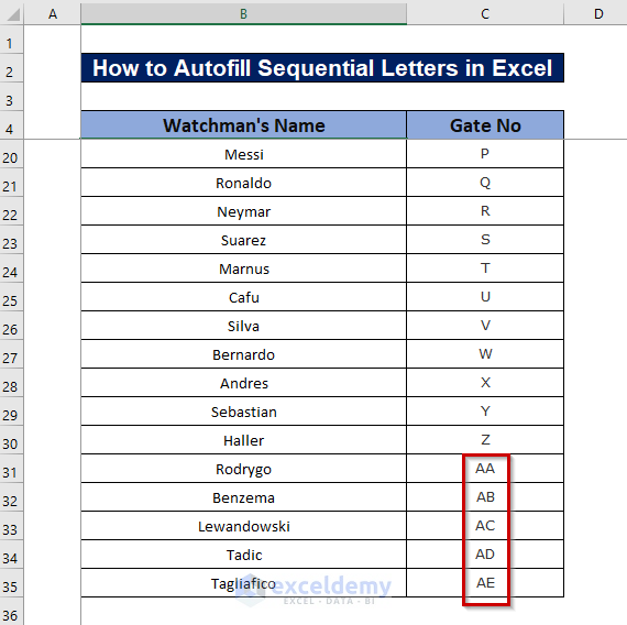
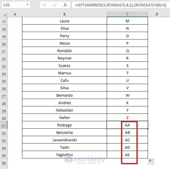
Again, when the value is greater than 26, sequential values of AB, AC, AD etc. will be filled.
Read More: How to Use Autofill Formula in Excel
Method 4 – Using Combined Functions
This combined function includes the IF, RIGHT, CHAR, CODE, LEFT, and MOD functions.
Steps:
- In cell C5 enter the first value, AB.
- Enter the following formula in cell C6:
=IF(RIGHT($C5,1)="Z",CHAR(CODE(LEFT(C5,1))+1),LEFT(C5,1))&CHAR(65+MOD(CODE(RIGHT(C5,1))+1-65,26))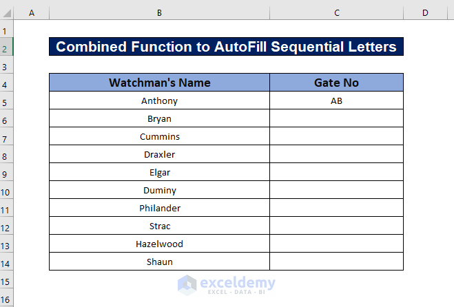
Formula Breakdown
- RIGHT($C5,1) —–> extracts 1 character from the right of the specified cell value.
- Output: B
- RIGHT($C5,1)=”Z”—–> checks if the second letter of the first input is equal to “Z” or not.
- “B”=”Z”
- Output: FALSE
- CHAR(CODE(LEFT(C5,1))) —–> returns a character based on its ASCII code value.
- CHAR(CODE(“A”))
- CHAR(65)
- Output: A
Note: If the output of RIGHT($C5,1)=”Z” is TRUE, then:
- CHAR(CODE(LEFT(C5,1))+1) —–> returns the character based on its ASCII code value.
- CHAR(CODE(“A”)+1)
- CHAR(65+1)
- CHAR(66)
- Output: B
Note: If the output of RIGHT($C5,1)=”Z” is FALSE, then:
- LEFT(C5,1) —–> extracts 1 character from the left side of the text.
- Output : A
- CHAR(65+MOD(CODE(RIGHT(C5,1))+1-65,26)) —–> becomes
- CHAR(65+MOD(CODE(RIGHT(“AB”,1))+1-65,26))
- CHAR(65+MOD(CODE(“B”))+1-65,26))
- CHAR(65+MOD(66+1-65,26))
- CHAR(65+MOD(67-65,26))
- CHAR(65+MOD(2,26))
- CHAR(65+2)
- CHAR(67)
- Output: C
- IF(RIGHT($C5,1)=”Z”,CHAR(CODE(LEFT(C5,1))+1),LEFT(C5,1))&CHAR(65+MOD(CODE(RIGHT(C5,1))+1-65,26))
- resolves to “A”&”C”
- Output: AC
- Press ENTER.
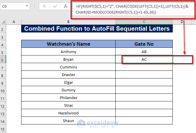
- To AutoFill the formula for the rest of the cells, use the Fill Handle.
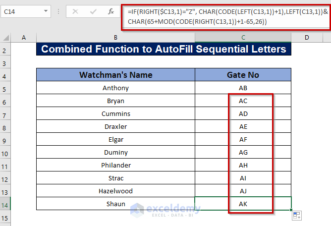
Read More: How to Apply AutoFill Shortcut in Excel
Method 5 – Using a User Defined Function
We can also use VBA to AutoFill sequential letters in Excel.
Steps:
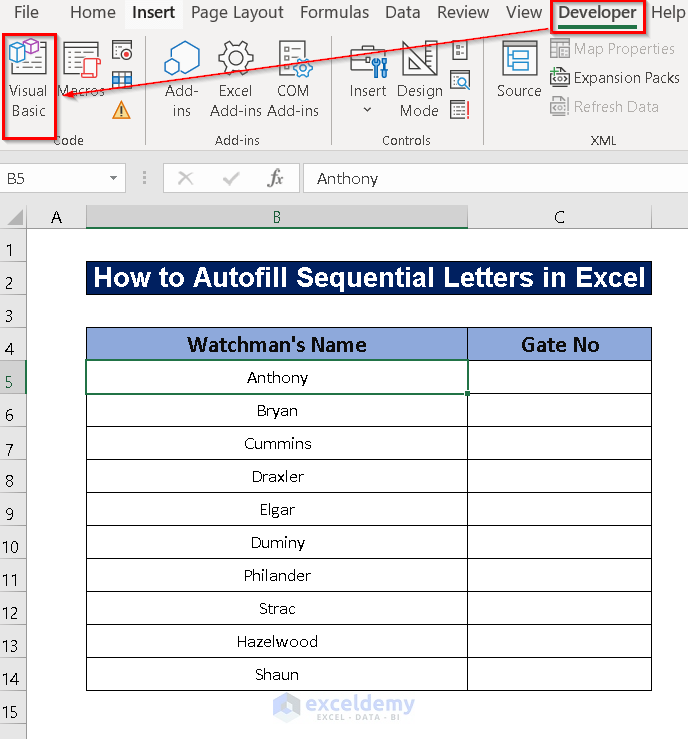
- Go to the Developer tab and select Visual Basic. Or press Alt + F11.
- From the Insert option, select Module.
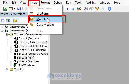
- Enter the following code in the Module:
Function AutoFill(b As Long) As String
AutoFill = Replace(Cells(1, b).Address(False, False), "1", "")
End Function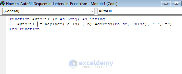
We’ve created a User Defined Function AutoFill, which uses the Replace.Address property to determine the cell value.
- Save the code and go back to the worksheet to use the function.
- Select cell C5 and enter the following formula:
=AutoFill(ROW())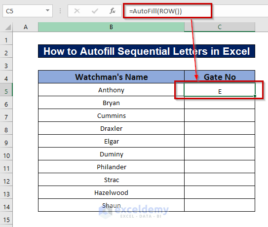
The result will be returned according to the row_num. As the row number of cell C5 is 5, the 5th letter is returned, namely E.
- Use the Fill Handle to AutoFill the rest of the cells.
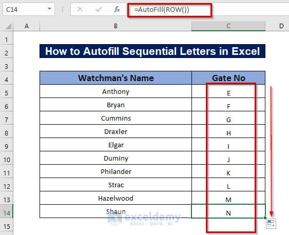
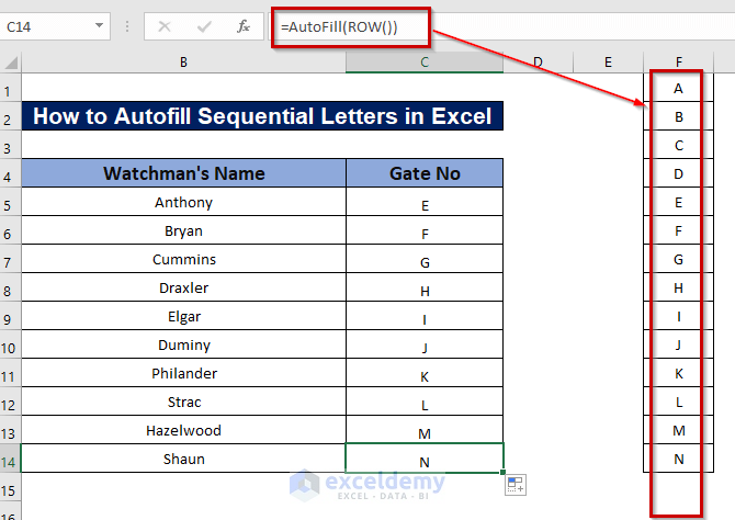
Read More: How to Create a Custom AutoFill List in Excel
Download Practice Workbook
Related Articles
- AutoFill Cell Based on Another Cell in Excel
- Fix: Excel Autofill Not Working
- [Fixed!] Auto Fill Options Not Showing in Excel
- [Solved:] Excel Double Click AutoFill Not Working
<< Go Back to Excel Autofill | Learn Excel
Get FREE Advanced Excel Exercises with Solutions!

