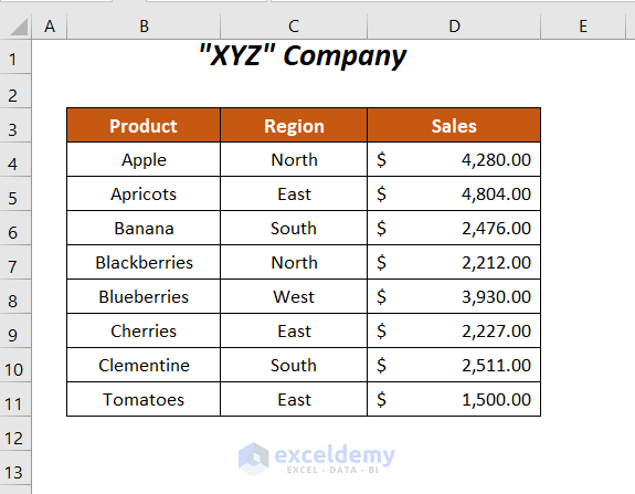
This is the sample dataset.
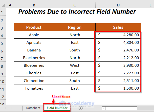
Solution 1 – Correcting the Field Number
Filter sales values greater than 2500:
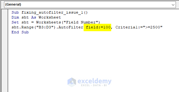
- Use this code:
Sub fixing_autofilter_issue_1()

Dim sht As Worksheet
Set sht = Worksheets("Field Number")
sht.Range("B3:D3").AutoFilter field:=100, Criteria1:=">=2500"

End Sub
Here, field: is the column number in the range, which was assigned to 100.
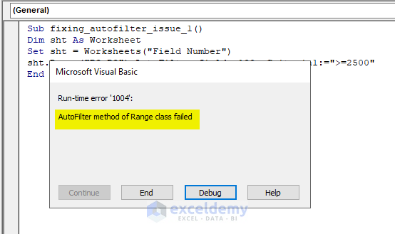
- Press F5 and the error message AutoFilter method of Range Class Failed will be displayed.
- Use the correct field number corresponding to the column number in the range (3, here– the serial number of the Sales column).
Sub fixing_autofilter_issue_1()

Dim sht As Worksheet
Set sht = Worksheets("Field Number")
sht.Range("B3:D3").AutoFilter field:=3, Criteria1:=">=2500"

End Sub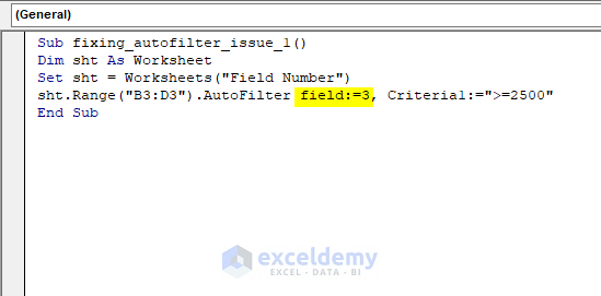
- Press F5.
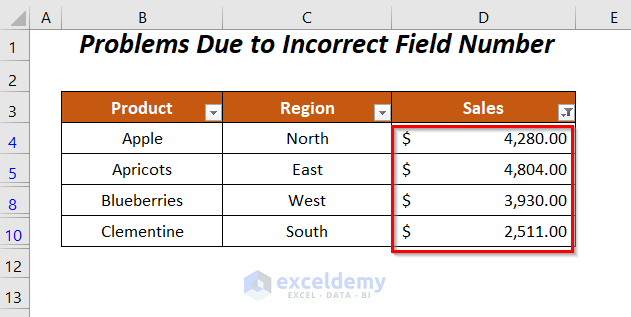
Filter your range. No error message will be displayed.
Read More: Excel VBA to Check If AutoFilter is On
Solution 2 – Using a Correct Range
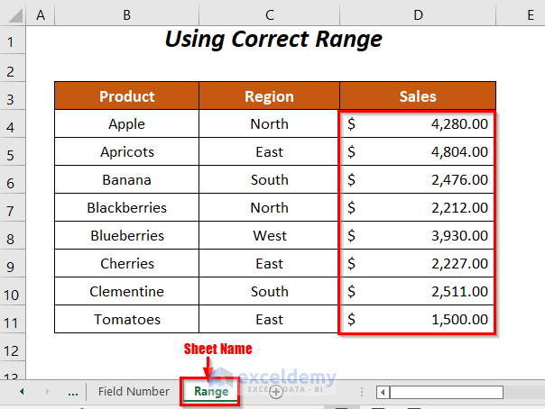
Filter the following dataset based on Sales values greater than $2,500.00:
- Use the following code.
Sub fixing_autofilter_issue_2()

Dim sht As Worksheet
Set sht = Worksheets("Range")
sht.Range("D3:D100").AutoFilter field:=3, Criteria1:=">=2500"

End Sub
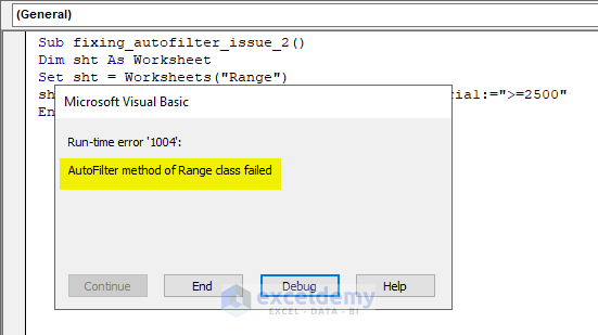
D3:D100 and the field number 3 do not match as this range contains one column only.
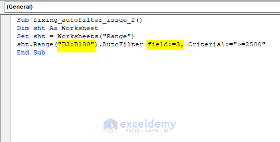
- Press F5 and the error message will be displayed.
- Change the code:
Sub fixing_autofilter_issue_2()

Dim sht As Worksheet
Set sht = Worksheets("Range")
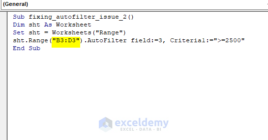
sht.Range("B3:D3").AutoFilter field:=3, Criteria1:=">=2500"

End Sub
The range changed to B3:D3.
- Press F5.
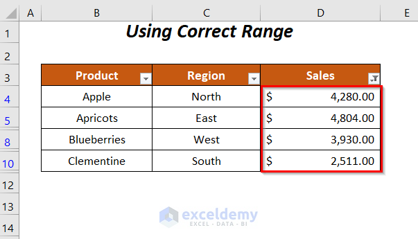
- Filter your range. No error message will be displayed.
Solution 3 – The AutoFilter Method of Range Class Failed Problem Due to a Filtering Table
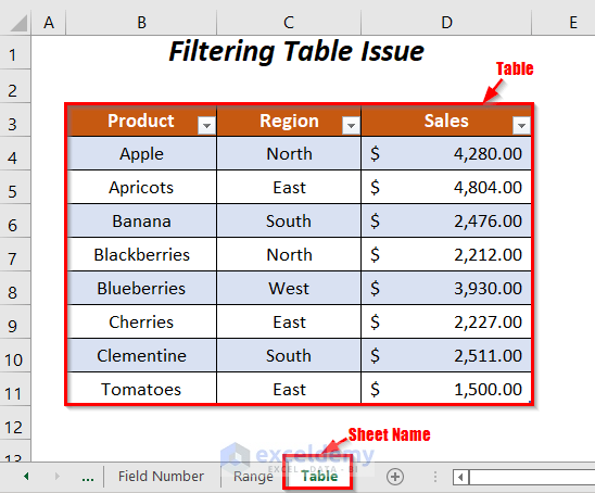
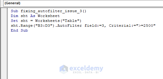
- Use the code:
Sub fixing_autofilter_issue_3()

Dim sht As Worksheet
Set sht = Worksheets("Table")
sht.Range("B3:D3").AutoFilter field:=3, Criteria1:=">=2500"

End Sub
This is the output.
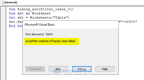
- Press F5 and the error message will be displayed.
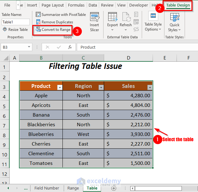
- Convert the table into a range.
- Select the table and go to Table Design >> Tools >> Convert to Range.
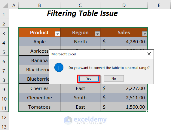
A message box will be displayed.
- Click Yes.
This is the output.
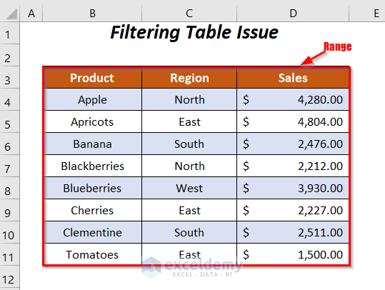
- Use the previous code again.
Sub fixing_autofilter_issue_3()

Dim sht As Worksheet
Set sht = Worksheets("Table")
sht.Range("B3:D3").AutoFilter field:=3, Criteria1:=">=2500"

End Sub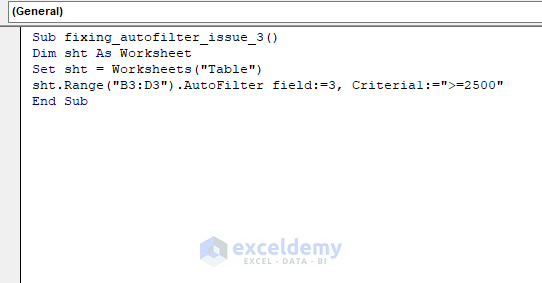
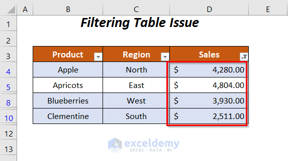
- Press F5.
This is the output.
Read More: VBA Autofilter: Sort Smallest to Largest
Solution 4 – AutoFilter Method of Range Class Failed Problem Due to Filtering a Pivot Table
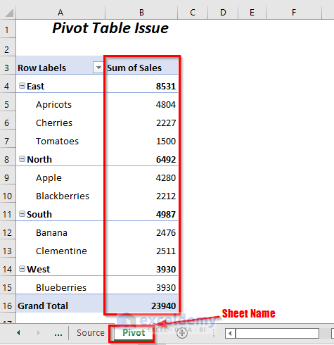
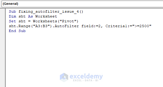
- Use the following code.
Sub fixing_autofilter_issue_4()

Dim sht As Worksheet
Set sht = Worksheets("Pivot")
sht.Range("A3:B3").AutoFilter field:=2, Criteria1:=">=2500"

End Sub
2 is the second column in A3:B3.
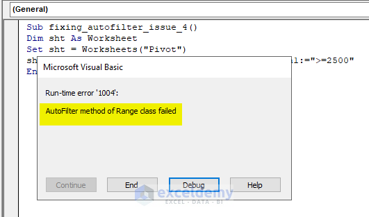
- After pressing F5, you will get the error message AutoFilter method of Range Class Failed.
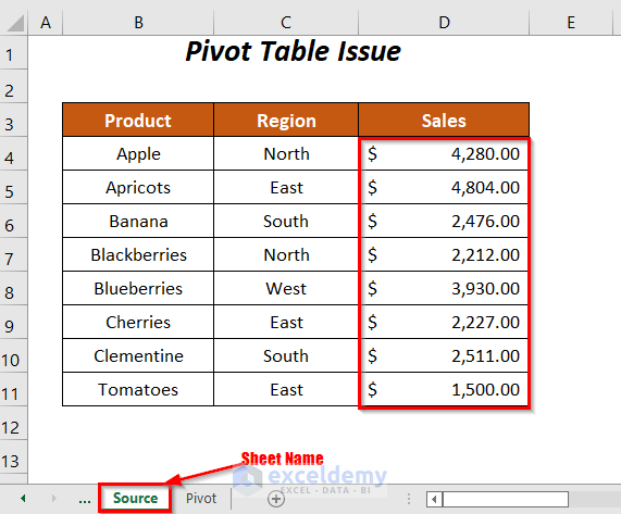
- Apply the AutoFilter method to the source range of the Pivot table.
- Enter the following code for this source range.
Sub fixing_autofilter_issue_4_1()

Dim sht As Worksheet
Set sht = Worksheets("Source")
sht.Range("B3:D3").AutoFilter field:=3, Criteria1:=">=2500"

End Sub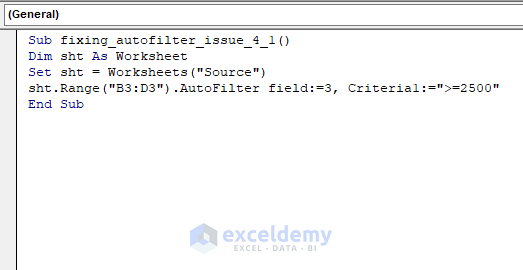
- Press F5.
You will be able to filter the range based on the given criteria.
Solution 5 – Using the Whole Range Instead of the Header
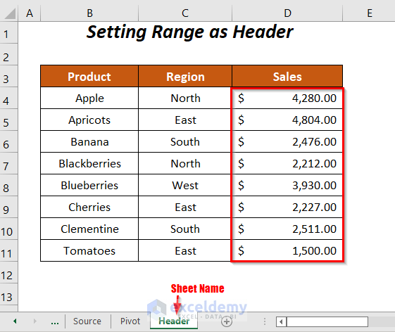
- Use the following code to apply the filter.
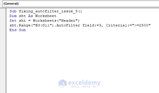
Sub fixing_autofilter_issue_5()

Dim sht As Worksheet
Set sht = Worksheets("Header")
sht.Range("B3:D11").AutoFilter field:=3, Criteria1:=">=2500"

End Sub
B3:D11 is the whole dataset and can cause an error message.
- Change the code and use the header as a range.
Sub fixing_autofilter_issue_5()

Dim sht As Worksheet
Set sht = Worksheets("Header")
sht.Range("B3:D3").AutoFilter field:=3, Criteria1:=">=2500"

End Sub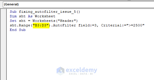
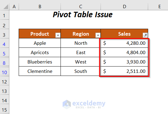
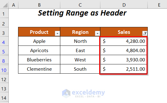
- After pressing F5, you will see the result.
Read More: Excel VBA: Remove AutoFilter If It Exists
Download Workbook
Related Articles
- How to Use Custom Autofilter in Excel for More Than 2 Criteria
- VBA to AutoFilter with Multiple Criteria on Same Field in Excel
- How to Autofilter Values Not Equal to a Certain Value with VBA in Excel


