How to Use the Average Attendance Formula in Excel (5 Methods)

Dataset Overview

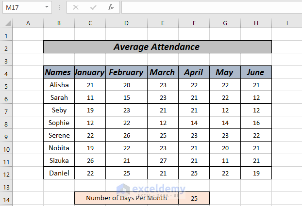
For your better understanding, we will use a sample dataset. The data set contains, Names, Months, Number of attendances, and number of total working days. We will calculate the average attendance per month, as well the average percentage per month. 

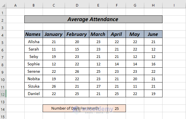
Method 1 – Average Attendance by Arithmetic Calculation

• In cell I5, enter the following formula:

• • This calculates the sum of attendance for six months and divides it by the total number of months (which is 6). We use an absolute cell reference for F15 to ensure consistent division.

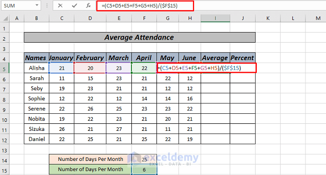
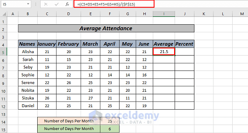
• Press ENTER.

• To calculate the percentage of attendance, enter this formula in cell J5:

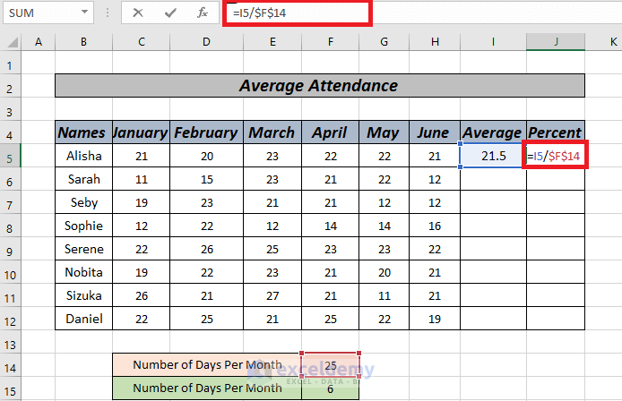
• Press ENTER.

• Use AutoFill to extend the formulas to the rest of the series.

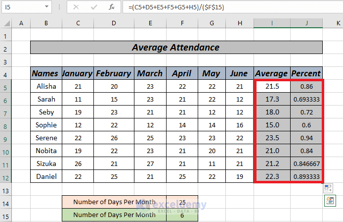
• Select the ranges in the percentage column from J5 to J12. 
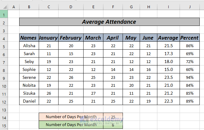
• Click the Percentage sign in the number tab.

• This will be the result.

Read More: How to Average Filtered Data in Excel

Method 2 – Average Attendance Using the Average Function

• Click on cell I5 and enter the following formula:

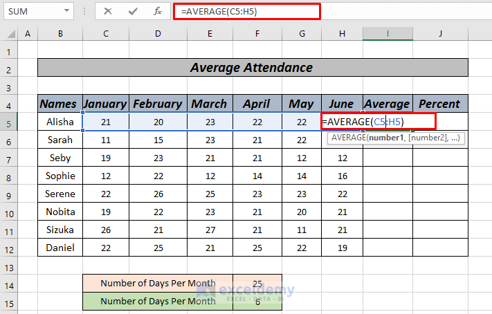
• This averages all values from C5 to H5.

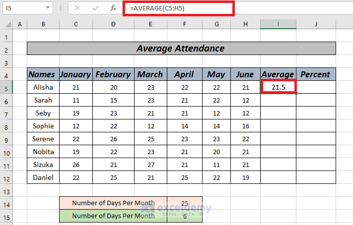
• Calculate the percentage of attendance in cell J5 using Method 1.

• Press ENTER.
• Use AutoFill to fill the rest of the series.

• Convert the percentage values in the Percent column by selecting the range and clicking the Percentage sign in the number tab.

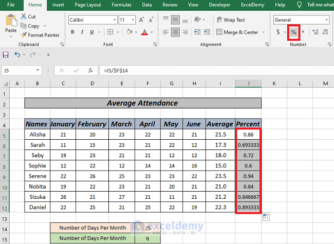
The data sheet is ready.

Read More: How to Calculate Class Average in Excel

Method 3 – Average Attendance Using Formula Ribbon

• Click on cell I5.
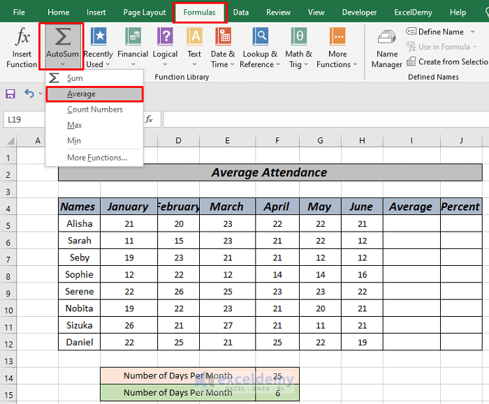
• Go to the Formulas ribbon and select Average from the AutoSum feature.

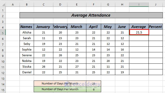
• Press ENTER.

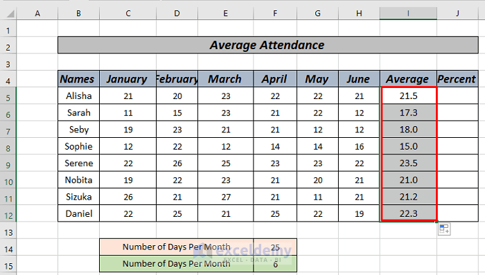
• Use AutoFill to complete the series.

Method 4 – Average Attendance Using a Shortcut Key

• If you’re comfortable with keyboard shortcuts, press ALT + M.

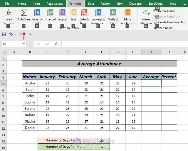
• Press U, then press A. Excel will automatically select the cells.

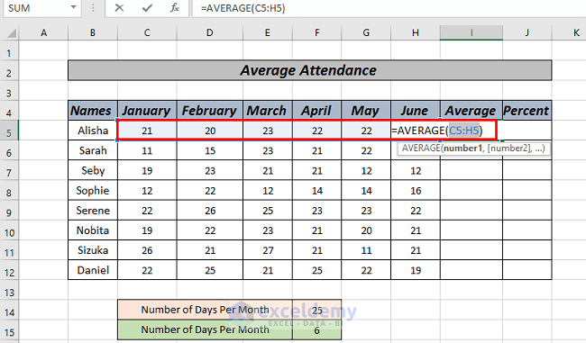
• Press ENTER.

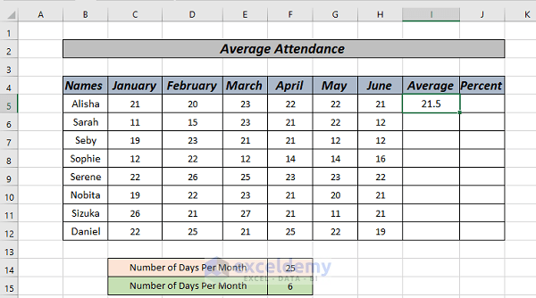
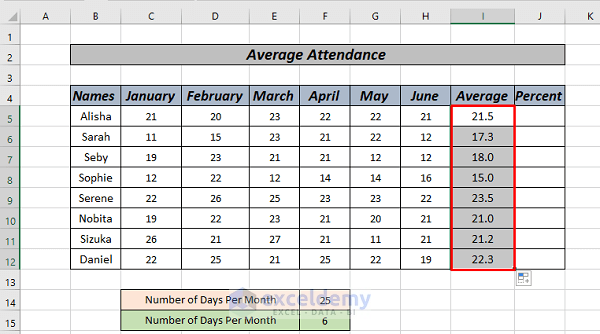
• Right-click and drag it down to AutoFill the series.

Related Content: How to Calculate Average Percentage of Marks in Excel

Method 5 – Average Attendance Using SUMPRODUCT Function in Excel

• Click on cell D12.
• Enter the following formula:
  
  =SUMPRODUCT(C5:C10,D5:D10)/SUM(C5:C10)

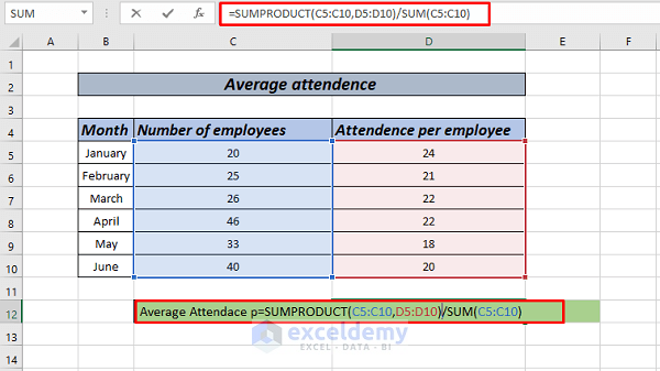
Here’s how it works:

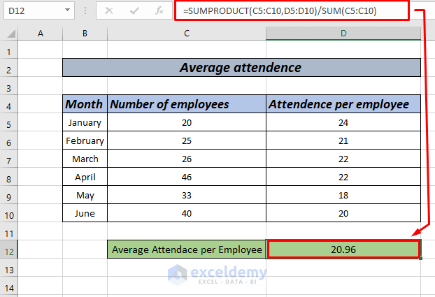
• • The SUMPRODUCT function calculates the sum of products for each month: (C5 * D5) + (C6 * D6) + … + (C10 * D10).
  • We then divide this sum by the total number of employees (SUM(C5:C10)).

• Press ENTER to get the results.

Practice Section

Feel free to practice using the provided sheet.

Download Practice Workbook

You can download the practice workbook from here:

Related Articles

• How to Calculate Average, Minimum And Maximum in Excel
• How to Calculate Average of Averages in Excel
• How to Calculate Average True Range in Excel
• How to Calculate Average Percentage in Excel
• How to Calculate Average Revenue in Excel
• How to Calculate Average Quarterly Revenue in Excel
• How to Calculate Average Share Price in Excel
• How to Calculate Average Length of Stay in Excel
• How to Calculate Average Price in Excel

<< Go Back to Excel Average Formula Examples | How to Calculate Average in Excel | How to Calculate in Excel | Learn Excel