What Is Variance Formula?
Actual variance is the difference between actual expenditure and budgeted expenditure.
We can calculate variance using two formulas; one for calculating the actual variance, and another for calculating the percentage variance.
The formula for actual variance is:
For the percentage variance, the formula is:
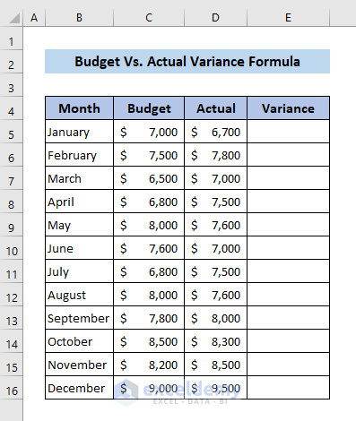
An Example of Budget vs Actual Variance Formula in Excel
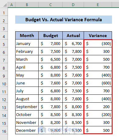
We have monthly budget amounts and actual sales amounts for a shop in our dataset below. Let’s calculate and depict the variance using this dataset.
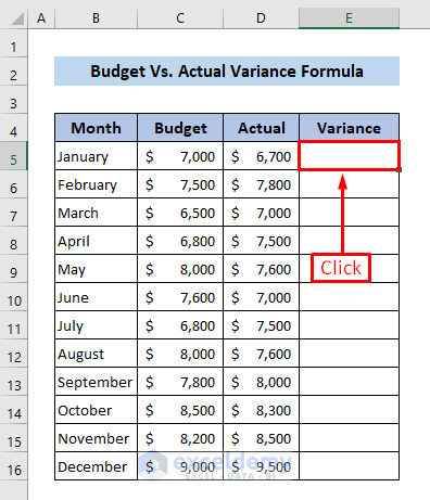
Steps:
- Click on cell E5, where the variance will be calculated.
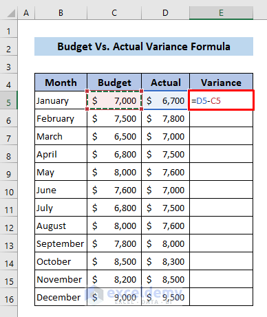
- Put an equal sign (=) and write D5-C5.
- Press Enter.
Read More: How to Calculate Semi Variance in Excel
The variance for January is returned.
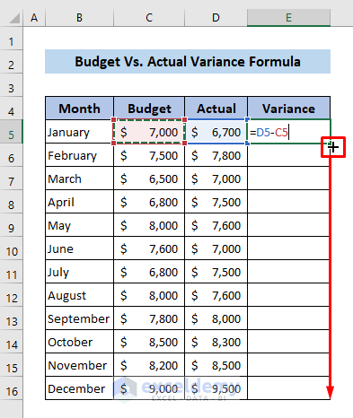
- Place your cursor in the bottom right position of the cell.
The Fill handle icon will appear.
- Drag it down to copy the formula to the cells below.
The budget vs actual variance in Excel for all months is complete.
Read More: How to Calculate Budget Variance in Excel
How to Create a Monthly Budget vs Actual Variance Chart
Now let’s plot the actual variance by month in a chart.
Steps:
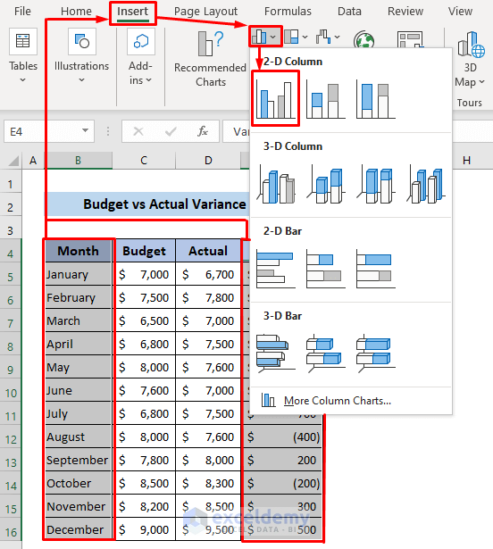
- Select the Month column and the Actual Variance column by holding the CTRL key while clicking on them.
- Go to the Insert tab >> click on the Insert Column or Bar Chart icon >> select the Clustered Column chart.
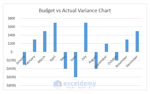
A chart is generated where the X-axis represents the month and the Y-axis represents the actual variance.
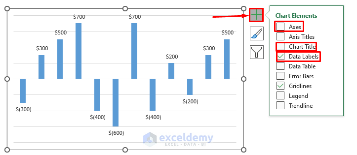
Let’s add some formatting to the graph to make it more presentable.
- Click on the chart area.
- Click on the Chart Elements icon on the right side of the chart.
- Untick the Axes and Chart Title options.
- Tick the Data Labels option.
For better visualization, let’s change the color of positive variances and negative variances.
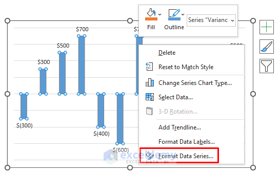
- Right-click on any column of the chart.
- Choose Format Data Series… from the context menu.
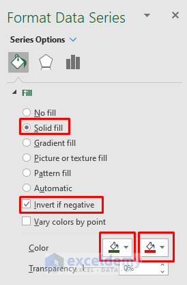
A new ribbon named Format Data Series opens on the right side of the Excel file.
- Click on the Fill & Line icon >> Fill group.
- Put the radio button on the Solid fill option.
- Tick the option Invert if negative.
- Choose two colors for a positive and negative variance from the Fill Color icons.
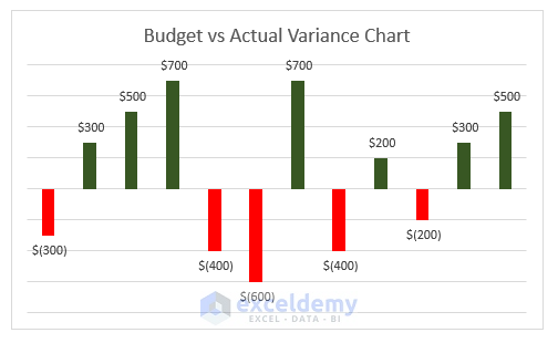
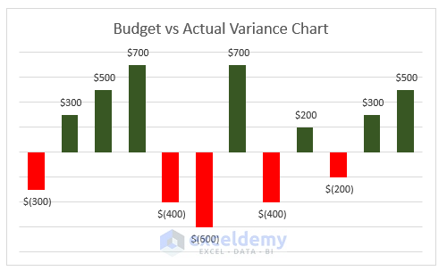
As we have chosen green as the first color and red as the second color, our chart will look like this.
We can also widen the columns for better visualization of the whole chart.
- As above, access the Format Data Series ribbon.
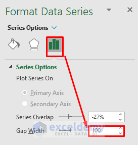
- Click on the Series Options icon >> Series Options group.
- Modify the Gap Width using the arrow buttons. For example, make it 100%.
Our chart is complete.
Read More: How to Create Minimum Variance Portfolio in Excel
Download Sample Workbook
Related Articles
- How to Calculate Portfolio Variance in Excel
- How to Calculate Variance of Stock Returns in Excel
- How to Do Price Volume Variance Analysis in Excel
- How to Calculate Schedule Variance Using Excel Formula
- How to Calculate Variance Inflation Factor in Excel
<< Go Back to Calculate Variance in Excel | Excel for Statistics | Learn Excel
Get FREE Advanced Excel Exercises with Solutions!
