Method 1 – Calculate Average Rating Using Multiplication and SUM function
Step 1:
- Go to Cell E5.
- Put the formula below, which is the multiplication of the Rating and of Customer.
=C5*D5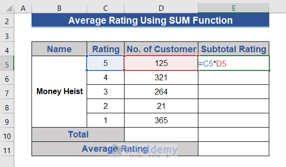
Step 2:
- Press Enter.
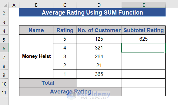
We get the subtotal of a 5-star rating.
Step 3:
- Drag the Fill Handle icon to Cell E9.
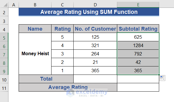
Step 4:
- We can perform this more easily. Put the following formula on Cell E5.
=D5:D9*C5:C9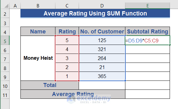
Step 5:
- Press the Enter button.
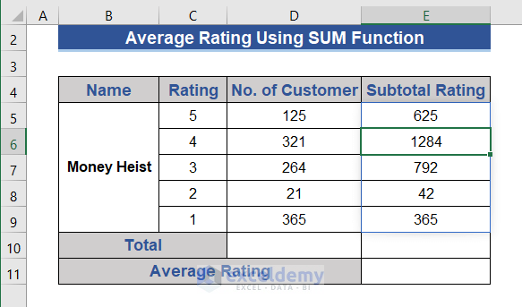
We do not need to apply the fill handle feature in this formula. We just put the whole range here.
Step 6:
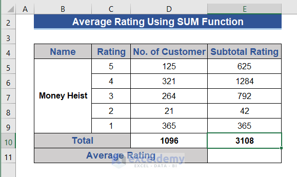
- Find the no. of the total customer using the following formula on Cell D10.
=SUM(D5:D9)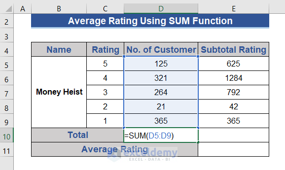
Step 7:
- Click the Enter button.
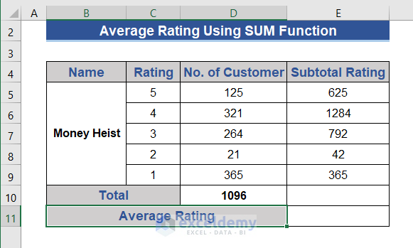
Step 8:
- Put another SUM formula on Cell E10 to the Total Rating.
=SUM(E5:E9)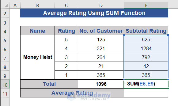
Step 9:
- Click on Enter.
Step 10:
- We get the total ratings and the total number of customers. Now, divide the total ratings by the total customers. Apply the following formula to Cell E11.
=E10/D10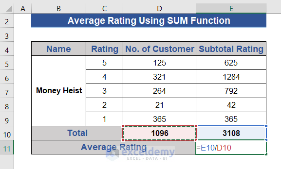
Step 11:
- Press the Enter button.
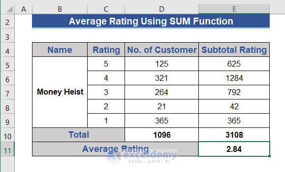
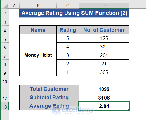
Our average rating is 2.84. We choose 2 decimal digits in the result.
Method 2 – Alternative Way for Average Rating Applying SUM Function Multiple Times
Step 1:
- Go to Cell D11.
- Put the following formula to get the total no. of customers.
=SUM(D5:D9)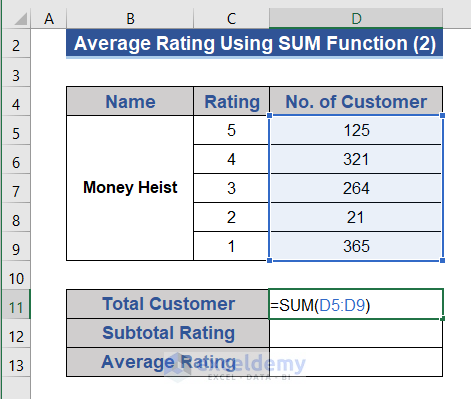
Step 2:
- Click the Enter button.
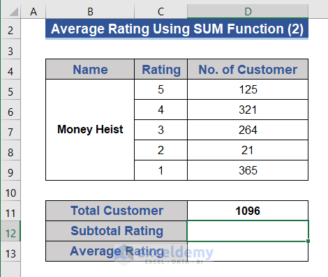
Step 3:
- Apply a SUM function to get the total ratings at Cell D12.
=SUM(C5:C9*D5:D9)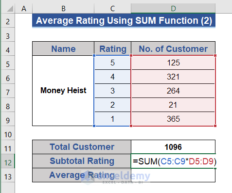
Step 4:
- Press the Enter button.
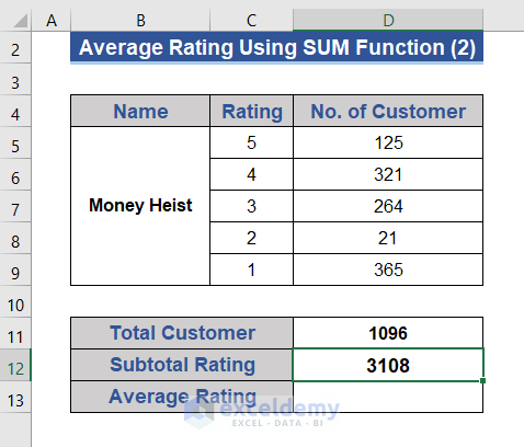
Step 5:
- Divide the total ratings by the total customer to get the average.
=D12/D11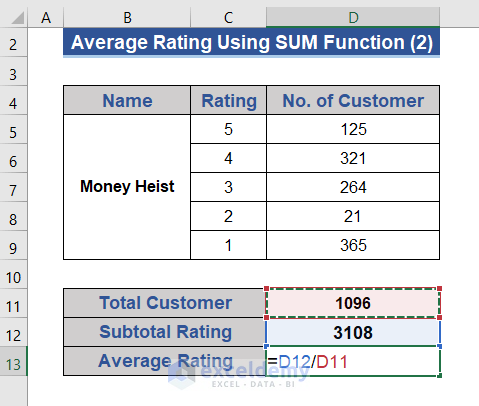
Step 6:
- Click the Enter button.
Method 3 – Insert SUMPRODUCT with SUM Function to Measure Average Rating
Step 1:
- Enter Cell D5.
- Put the formula below to get the total customer.
=SUM(D5:D9)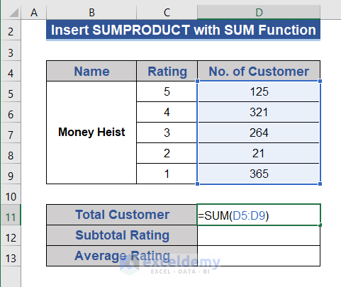
Step 2:
- Press the Enter button.
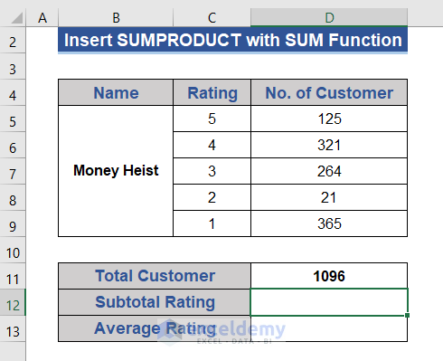
Step 3:
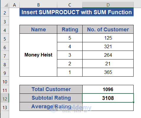
- Apply the SUMPRODUCT based function on Cell D12.
=SUMPRODUCT(C5:C9,D5:D9)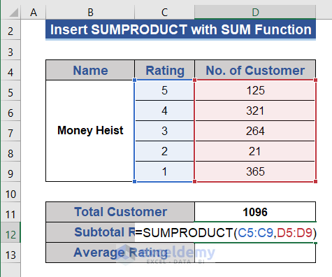
Step 4:
- Click the Enter button.
Step 5:
- Go to Cell D13.
- Write the following formula to divide the total ratings by the total customers.
=D12/D11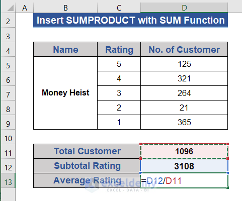
Step 6:
- Press the Enter button.
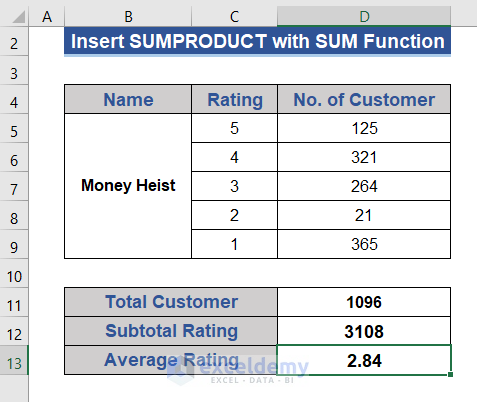
This average rating is calculated by inserting the SUMPRODUCT function with the SUM function.
Method 4 – Combination of SUM and COUNT Functions for Average Rating
The combination of SUM and COUNT functions is used in different situations. When we have only the raw data of the review, this combination is more useful than the others.
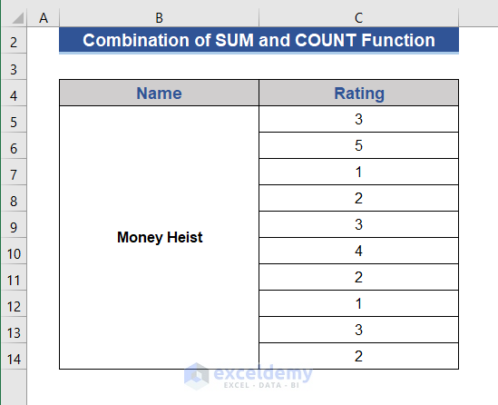
We add 3 rows in the dataset for calculation.
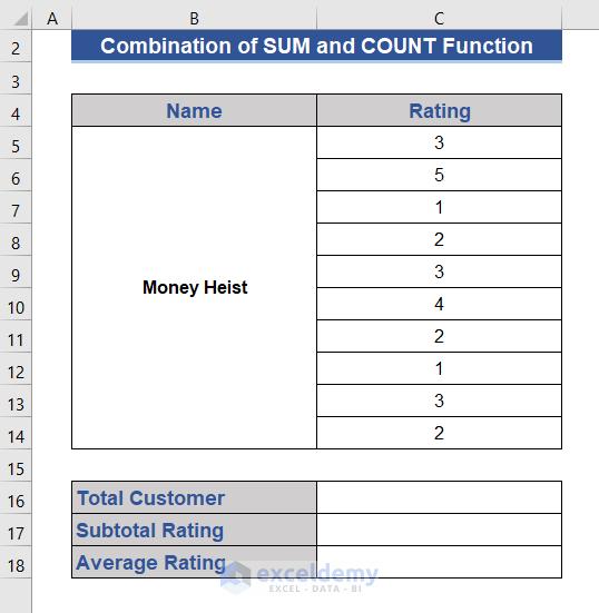
Step 1:
- Count the total number of customers. Go to Cell C16.
- Write the formula below.
=COUNT(C5:C14)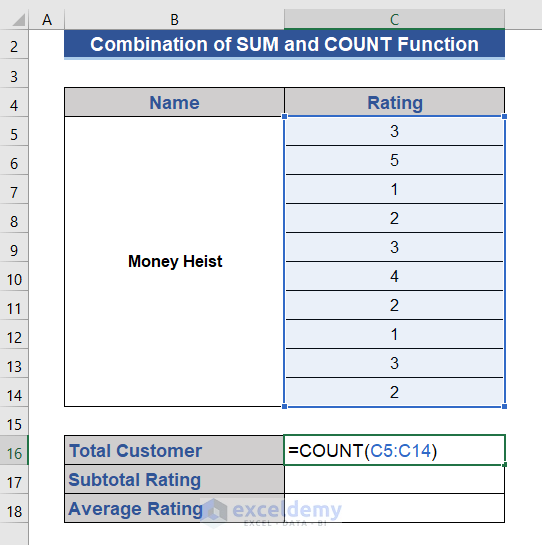
Step 2:
- Press the Enter button.
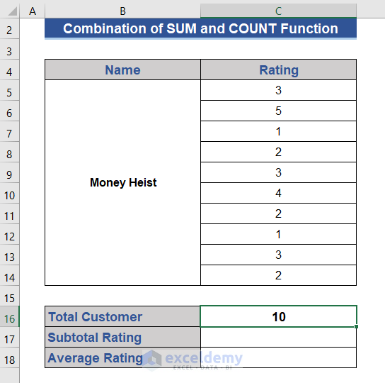
This formula counts total customers from the Rating column.
Step 3:
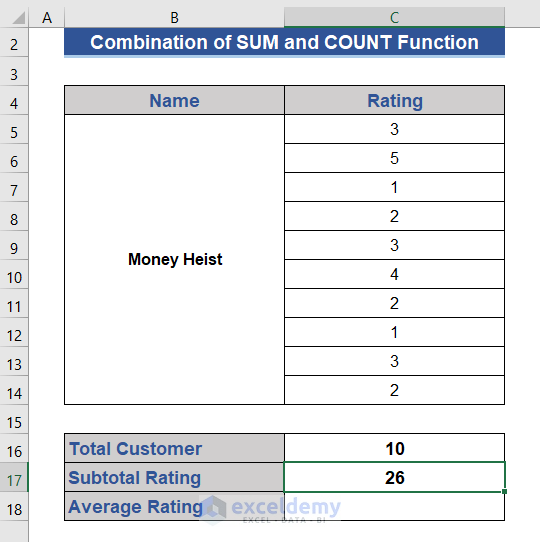
- Go to Cell C17.
- Put the formula below to get total ratings.
=SUM(C5:C14)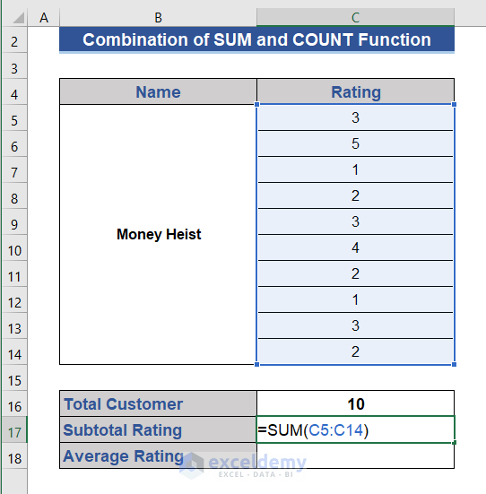
Step 4:
- Click the Enter button.
Step 5:
- Enter Cell C18 to get the average applying the following formula.
=C17/C16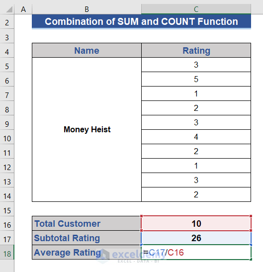
Step 6:
- Press the Enter button.
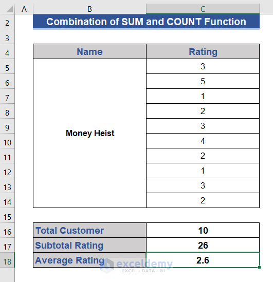
We have a total of 10 viewers who gave the rating and got the average rating.
Method 5 – Insert AVERAGE Function to Calculate Average Rating
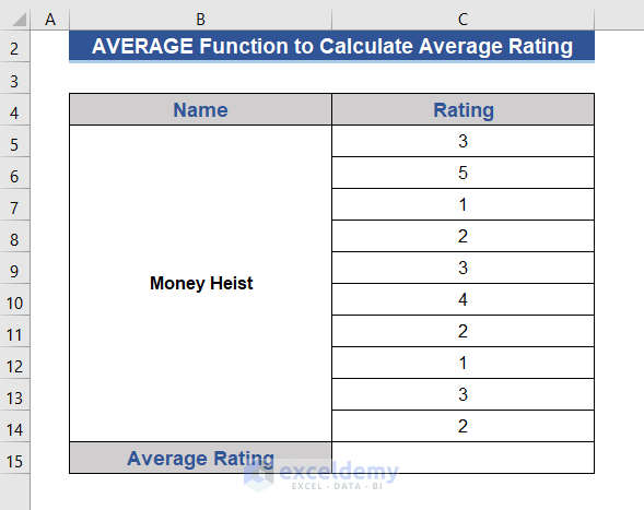
Apply the AVERAGE function to calculate the average rating. We are considering the dataset below for this example.
Step 1:
- Go to Cell C15.
- Write the following formula based on the AVERAGE function.
=AVERAGE(C5:C14)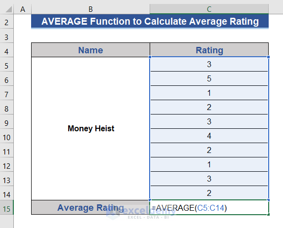
Step 2:
- Press Enter.
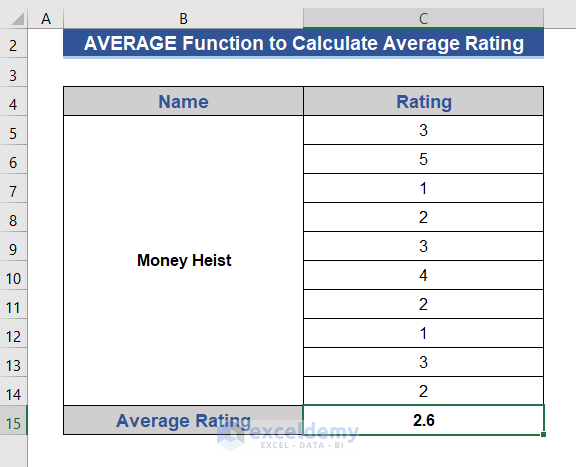
We calculated the average rating here.
Method 6 – Apply Excel AutoSum Tool to Determine Average Rating
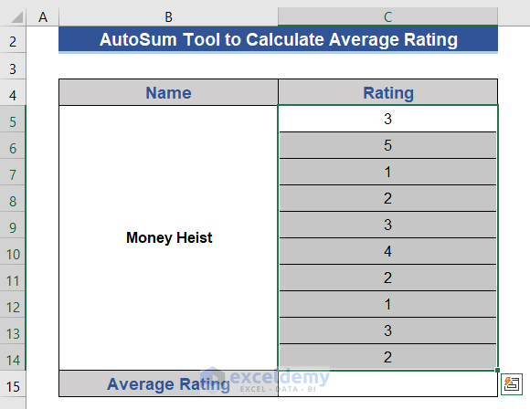
Step 1:
- Select all the cells containing ratings.
Step 2:
- Go to the Editing group from the Home tab.
- Select the Average feature from the AutoSum tool.
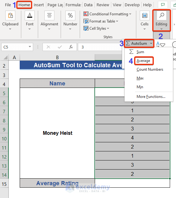
Look at Cell C15.
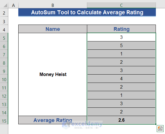 The average rating is shown here.
Method 7 – Excel VBA to Calculate Average Rating
Apply a VBA Macro code to calculate the average rating for the dataset given below.
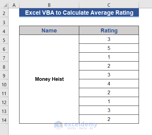
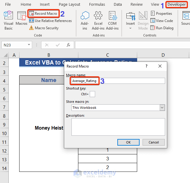
Step 1:
- Go to the Developer tab.
- Click on Record Macro.
- Put a name for the Macro and press OK.
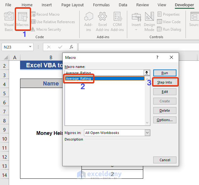
Step 2:
- Go to the Macros field.
- Select Average_Rating macro and Step Into it.
Step 3:
- Write the following VBA code on the command module.
Sub Average_Rating()
 Dim data As Range
 Dim total_rating, total_viewers As Integer
 Dim rating As Double
  Set data = Application.InputBox("Select Range", "Input Section", Type:=8)
  total_rating = WorksheetFunction.Sum(data)
  total_viewers = WorksheetFunction.Count(data)
  rating = total_rating / total_viewers
  MsgBox ("The Average Rating is " & rating)
End Sub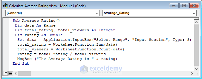
Step 4:
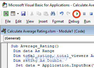
- Click on the marked box to run the code or press F5.
Step 5:
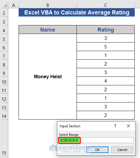
- In the Input Section window select our desired range.
- Press OK.
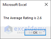
Look at the result.
Things to Remember
- Carefully select the cell references.
- When applying AutoSum first select the desired range
Download Practice Workbook
Download this practice workbook to exercise while you are reading this article.
Related Articles
- How to Calculate Average Growth Rate in Excel
- How to Get Average Time in Excel
- How to Calculate Daily Average in Excel
- How to Calculate Daily Average from Hourly Data in Excel
- How to Calculate Weekly Average in Excel
- How to Calculate Monthly Average from Daily Data in Excel
<< Go Back to Excel Average Formula Examples | How to Calculate Average in Excel | How to Calculate in Excel | Learn Excel
Get FREE Advanced Excel Exercises with Solutions!

