How to Calculate Elapsed Time in Excel (5 Ways)

Method 1 – Calculate Elapsed Time in Excel by Subtracting Two Date Values

In this example, we’re going to calculate the elapsed time of World War 2. Here, cells B3 and C3 contain the starting and ending date of the war with time. In cell C5, we subtracted cell B3 from cell C3.

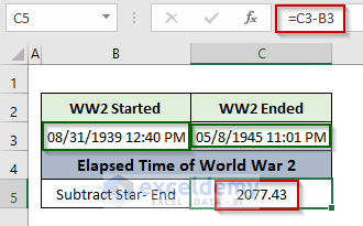The subtraction returned a number that is not meaningful. It represents the difference in serial numbers of these two dates. Excel stores date as a serial number that starts from 1 at the date 1/1/1900. So, this output number means there was a total of 2077.43 days elapsed in WW2.

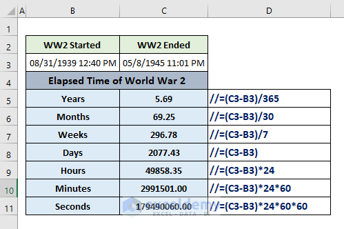
Now, we can calculate:

Years by dividing the number of days(output) by 365,
Months by dividing the number of days (output) by 30,
Weeks by dividing the number of days (output) by 7,
Hours by multiplying the number of days (output) with 24
Minutes by multiplying the number of days (output) with 24*60,
Seconds by multiplying the number of days (output) with 24*60*60.

Method 2 – Estimating Elapsed Time in Excel Using the TODAY, NOW, NETWORKDAYS Functions

Case 2.1 Use of the TODAY Function

Here in cell C3, we stored the starting date of the Summer Olympics 2024.

In cell C4, we used the following formula to find the number of days left to start Olympic 2024 from today’s date:

=(C3-TODAY())

We calculated the number of months and weeks by dividing the days’ number by 30 and 7 respectively in cells C5 and C6. To find out the number of years left, we used the YEAR function in cell D6. The formula is:

=(YEAR(C3)-YEAR(TODAY()))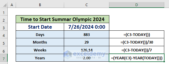

Case 2.2 Use of the NOW Function

The NOW function returns the current date and time displayed in the Excel worksheet. In this example, we used this function to calculate hours, minutes, and seconds left to begin the Summer Olympics 2024.

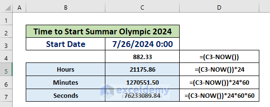
Case 2.3 Use of the NETWOKDAYS Function

The NETWORKDAYS function calculates the number of working days of a given time interval assuming 5 working days in a week starting on Monday.

Method 3 – Compute Elapsed Time Using the TEXT Function in Excel

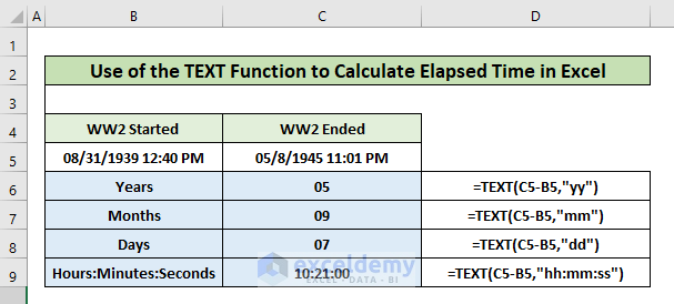
The TEXT function in Excel converts a numeric value to text and displays it in a specific predefined format. The function takes two arguments: value and format_text.

In this example, we put the difference between the ending and starting dates of WW2 as the value argument and different formats to display the duration of the war in years, months, days, hours, minutes, and seconds. Here, cells C5 and B5 contain the ending and starting dates respectively.

Method 4 – Use of Custom Formatting to Calculate Elapsed Time in Excel

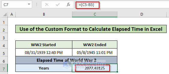
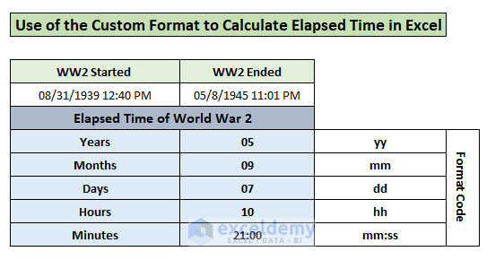
In cell C7, we calculated the difference between two dates in cells C5 and B5, which are the ending and starting dates of WW2. The output is the serial number difference of the input dates.

To show the year difference of these two dates, follow the steps below.

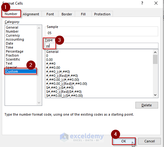
Steps:

Select cell C7 and press Ctrl + 1 to open the Format Cells
Go to the Number
Select the Custom
Type yy in the input box.
Hit OK.

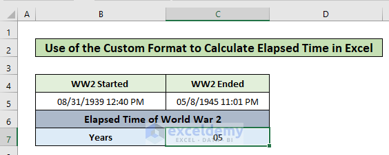
The output is the number of years elapsed in World War 2.

Similarly, we can calculate the other values using the different format codes shown in the below screenshot.

Method 5 – Handle Negative Values in Elapsed Time

If the end time is less than the start time, we cannot subtract normally to get the time difference. To handle this negative time, we can follow two ways.

Case 5.1 Use of Conditional IF Statement

Apply the following formula in cell D4, where C4 contains the end time and B4 contains the start time:

=IF(C4<B4,1+C4-B4,C4-B4)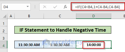

In this formula, we used the conditional IF statement to set the logic of whether the end time is less than the start time. If the logic returns TRUE, then it’ll add 1 with the time difference of two times assuming the clock running for a full 24-hour period.

Case 5.2 Use of the MOD Function

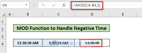
The MOD function can easily handle the above situation. The function changes the negative number to a positive one as it works for both the time in the same day and the time that spans midnight. We just need to use 1 as the divisor (2nd argument).

Things to Remember

The NETWORKDAYS function excludes Saturday and Sunday from a week while calculating the workdays between two dates.
If we want to add a custom holiday list to calculate the working days between two dates, we need to use the INTL function.

Download Practice Workbook

Download this practice workbook to exercise while you are reading this article.

Elapse Time in Excel.xlsx

Related Articles