This article will describe how to calculate home loan Interest in Excel. Suppose we have a dataset in column B containing the Total Loan Amount, Interest Rate, Period Term in Months, and Compounding Periods Per Month. Using this information, we’ll calculate the Total Interest on our home loan using 2 different methods.
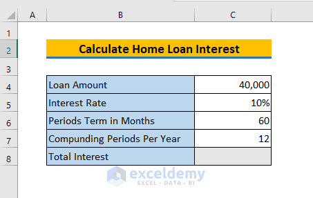
Method 1 – Using the Generic CUMIPMT Function
We can easily calculate the total home loan interest by using the CUMIPMT function in Excel. We’ll use this function to calculate every year-end interest on the home loan, then add them to calculate the total interest.
Steps:
- Create a new data table with two columns F and G representing the respective years and interest.
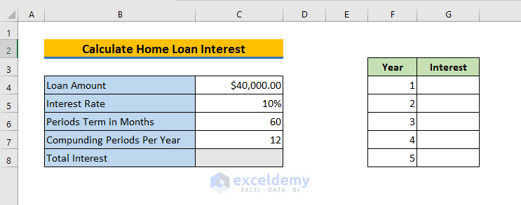
To calculate the interest after the 1st year:
- In cell G4, enter the following formula:
=CUMIPMT(rate,nper,pv,start,end,type)In this example, we will calculate the total interest for each year on a 5-year loan of $40,000 with a fixed interest rate of 10%. So, we apply CUMIPMT like this:
rate – refers to the interest rate per period. We divide the annual interest rate of 10% by 12 to get the monthly interest rate.
nper – refers to the total number of payment periods for the loan, here 12 * 5 = 60.
pv – refers to the present value, or the total value of all payments to date, namely $40000.
start_period – refers to the starting period for the given year.
end_period – refers to the ending period for the given year.
So, for year 1, the formula is:
=CUMIPMT(5%/12,60,30000,1,12,0)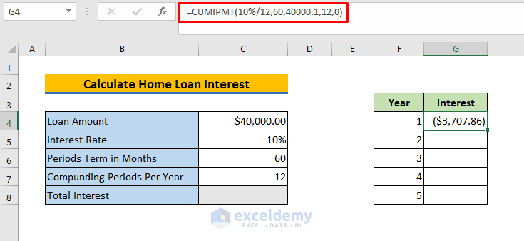
- Press ENTER to return the 1st year-end interest.
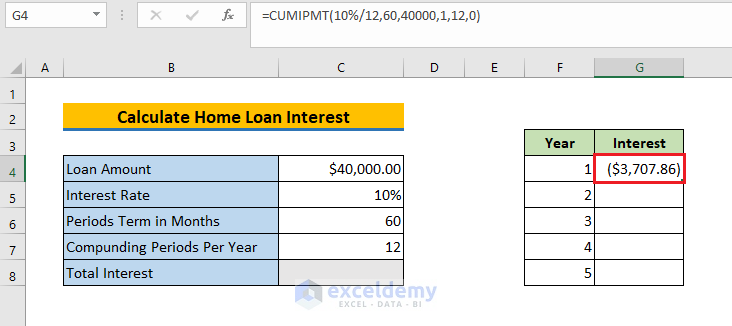
- Apply the same formula in the range G5:G8 to calculate the other year-end interests. The formulas are:
=CUMIPMT(10%/12,60,40000,13,24,0) // year 2 =CUMIPMT(10%/12,60,40000,25,36,0) // year 3
=CUMIPMT(10%/12,60,40000,37,48,0) // year 4
=CUMIPMT(10%/12,60,40000,49,60,0) // year 5
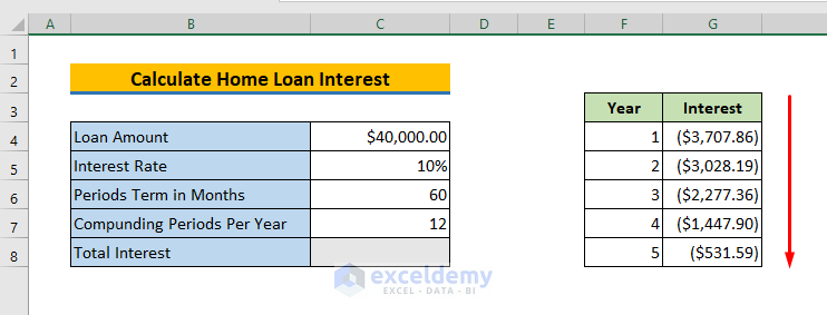
Now in cell C8, we’ll calculate the total home loan interest using the SUM function.
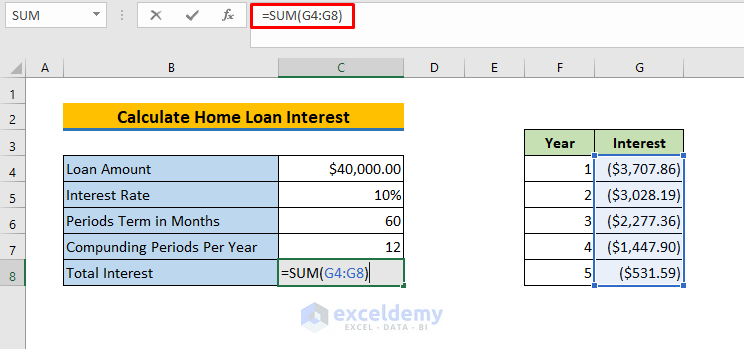
- Enter the following formula in cell C8:
=SUM(G4:G8)Here, G4:G8 is the range where all 5 years’ interest amounts are stored.
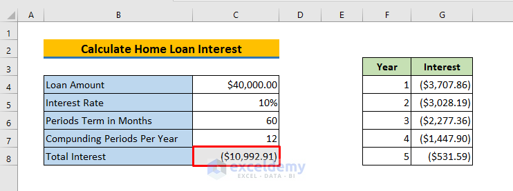
After pressing ENTER, the total interest is returned.
Read More: How to Calculate Interest on a Loan in Excel
Method 2 – Using a Known EMI Value
We can calculate the total home loan interest in Excel without having the interest rate, and only having the known Loan Amount, Period Term in Months, Compounding Periods Per Month, and the EMI Value.
Steps:
- Select cell C8.
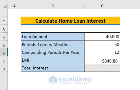
- Enter the following formula:
=C7*C5-C4Here, C7*C5 represents the total amount that will be paid after 5 years including interest. We then subtract the loan amount to get the total interest.
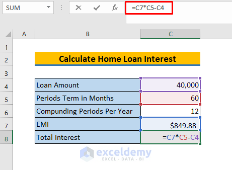
- Press ENTER to return the total interest.
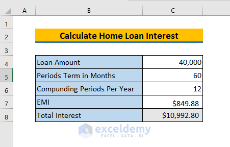
Read More: How to Calculate Gold Loan Interest in Excel
Download Practice Workbook
Related Articles
- How to Calculate Principal and Interest on a Loan in Excel
- How to Calculate Credit Card Interest in Excel
- How to Calculate Accrued Interest on Fixed Deposit in Excel
- How to Calculate Accrued Interest on a Bond in Excel
- How to Calculate Accrued Interest on a Loan in Excel
<< Go Back to Excel for Finance | Learn Excel
Get FREE Advanced Excel Exercises with Solutions!

