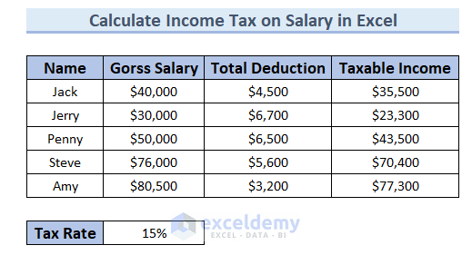
In this article, we will demonstrate different methods to calculate Income Tax on Salary. To illustrate our methods, we’ll use the following sample dataset that contains Employee Name, Gross Salary, and Taxable Income for different employees.
Example 1 – Using Generic Formula
The simplest way to calculate income tax in Excel is using the generic formula. We’ll use a fixed tax rate for all the employees and calculate the income tax on their salaries.
Steps:
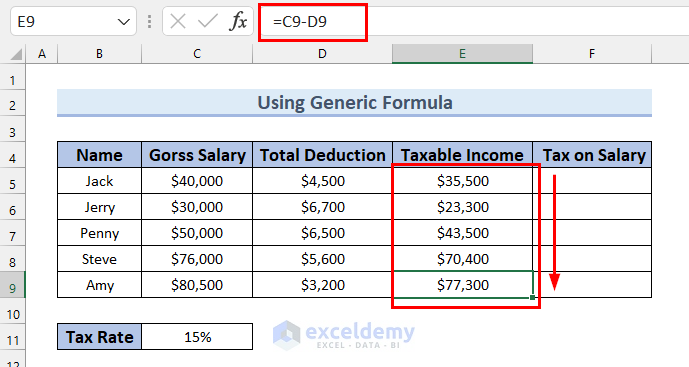
First, we calculate taxable income from the Gross Salary and Total Deduction.
- Select the cell in which to calculate the taxable income (cell E5).
- Enter the following formula:
=C5-D5 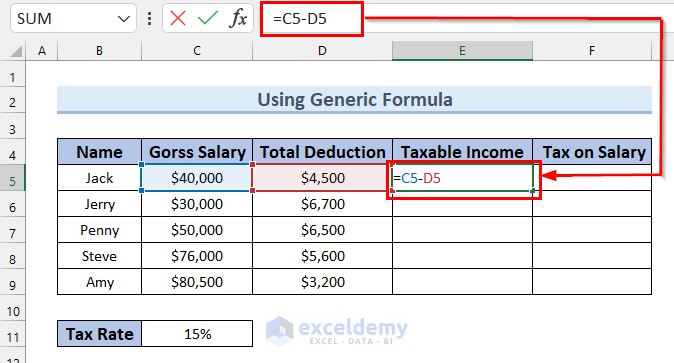
Here, we simply subtract the Total Deduction from the Gross Salary.
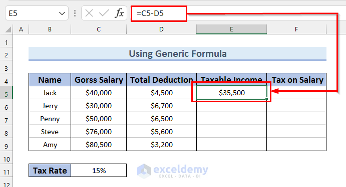
- Press ENTER to return the Taxable Income for Jack.
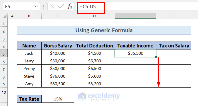
- Drag the Fill Handle down to get Taxable Income for every employee.
Now, we can calculate the Tax on Salary.
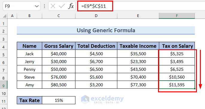
- Select the cell in which to calculate the Tax on Salary (cell F5).
- Enter the following formula:
=E5*$C$11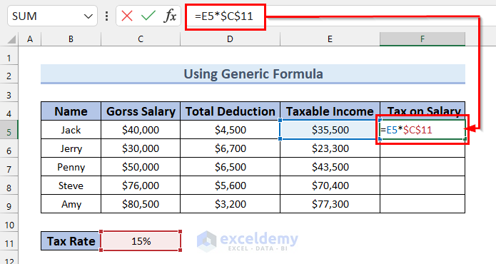
Here, E5 is the Taxable Income for that particular employee and C11 is the fixed Tax Rate. We multiply Taxable Income by Tax Rate to get that employee’s Tax on Salary.
- Press ENTER.
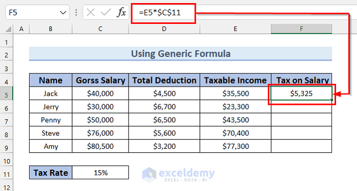
- Drag the Fill Handle down to get Tax on Salary for every employee.
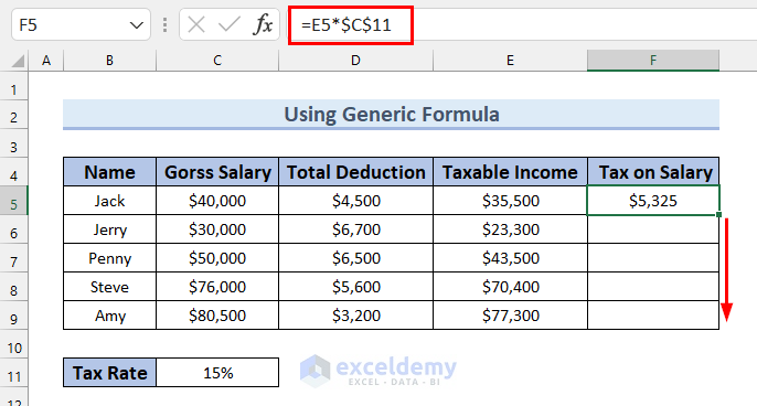
The results are as follows:
Read More: Reverse Tax Calculation Formula in Excel
Example 2 – Different Tax Brackets and Tax Surcharge
Now let’s calculate the tax on salary when where there are different tax brackets (also called slabs) for different income ranges, and a surcharge is applied on the tax for some income ranges.
Steps:
- In cell D5 enter the following formula:
=C5*C13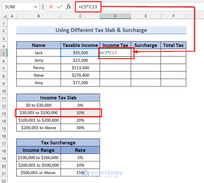
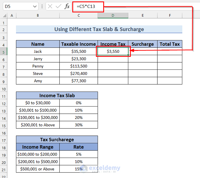
Here, C5 is the Taxable Income for Jack and C13 is the tax rate from the Income Tax Slab for that particular income range. The formula will multiply these two values and return the Income Tax for that employee.
- Press ENTER to return the Income Tax for Jack.
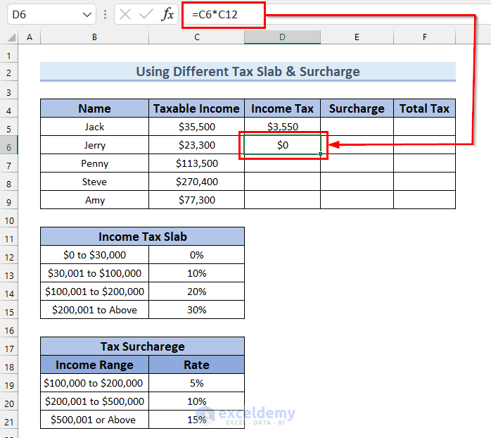
- In cell D6 enter the following formula:
=C6*C12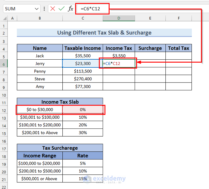
Here, C6 is the Taxable Income for Jack and C12 is the tax rate from Income Tax Slab for that particular income range. This formula will multiply these two values and return the Income Tax for Jack.
- Press ENTER.
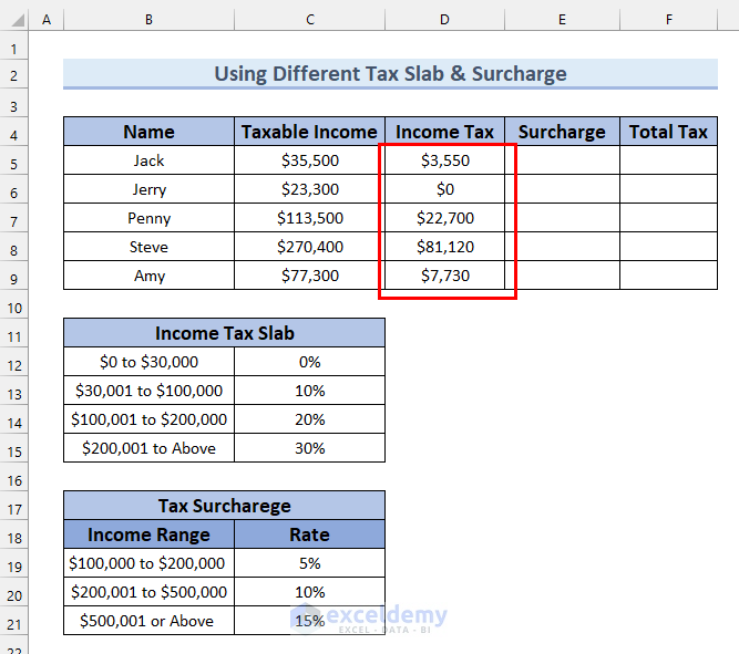
- Calculate Income Tax for every employee by following these exact steps.
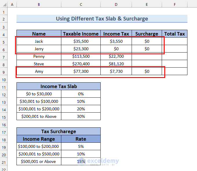
In our dataset, a Surcharge is applied on the tax for some income ranges. No surcharge is applicable for Jack, Jerry, and Amy, because their Taxable Income does not fall in those ranges.
For Penny, a 5% surcharge is applicable. Let’s calculate her Surcharge.
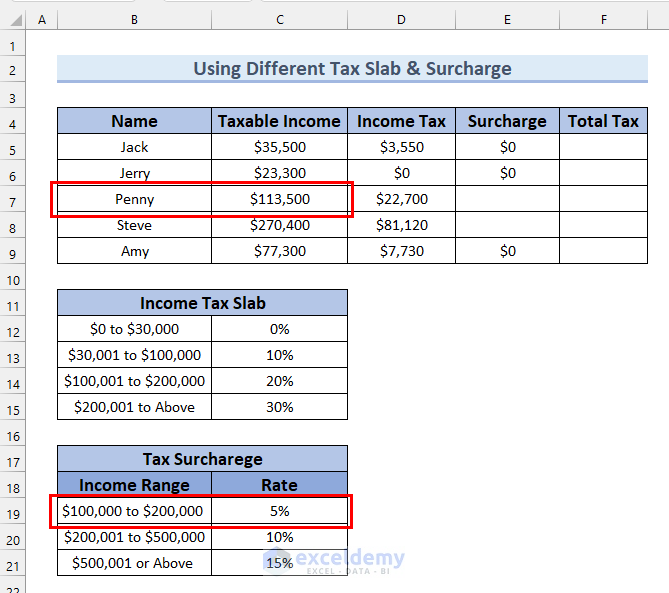
- In cell E7, enter the following formula:
=D7*C19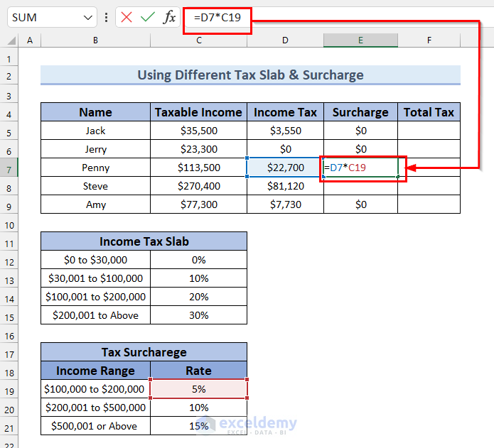
Here, D7 is the Income Tax for Penny and C19 is the Surcharge Rate. This formula will multiply Income Tax and Rate and return the Surcharge on tax for Penny.
- Press ENTER.
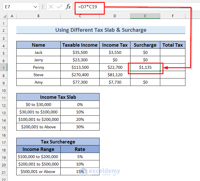
For Steve, a 10% surcharge is applicable.
To derive Steve’s Surcharge, we’ll follow the same steps as we followed for Penny.
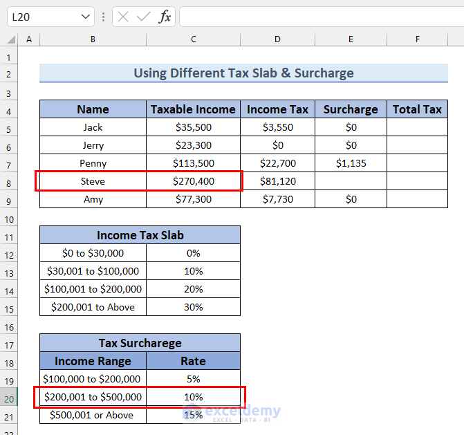
- In cell E8, enter the following formula:
=D8*C20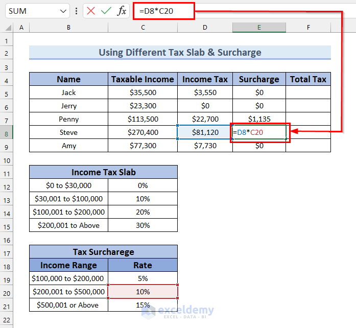
Here, D8 is the Income Tax for Steve and C20 is the Surcharge Rate. This formula will multiply Income Tax and Rate and return the Surcharge on tax for Steve.
- Press ENTER.
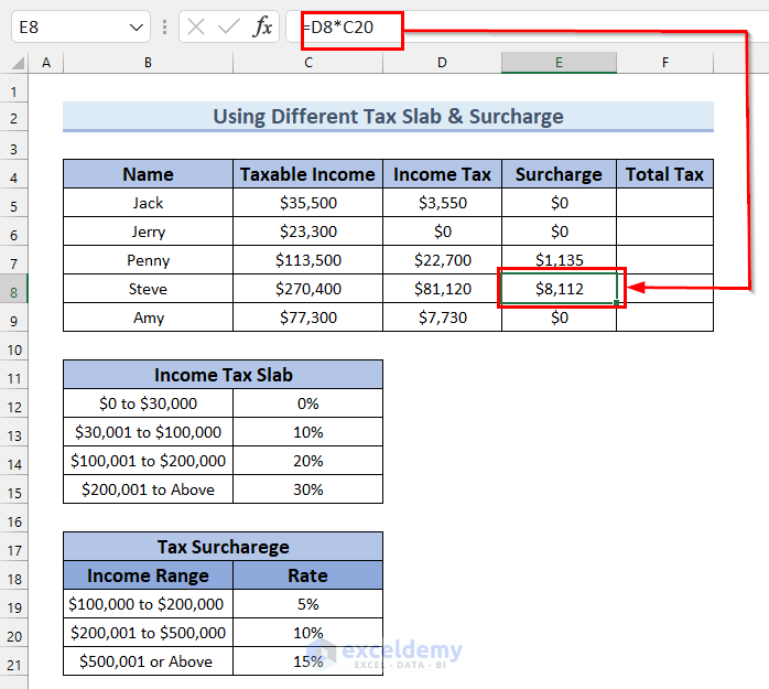
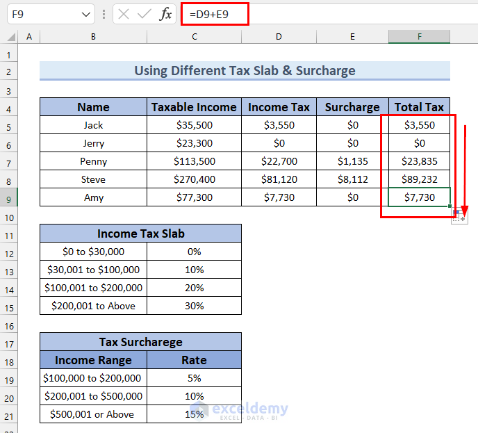
Now that we have income tax and surcharge for all the employees, we can calculate the total tax for every employee.
- In cell F5, enter the following formula:
=D5+E5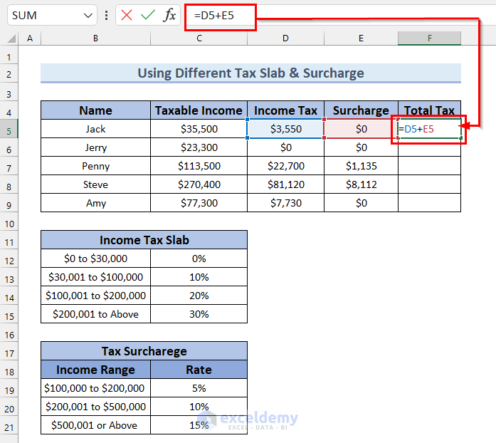
Here, D5 is Income Tax and E5 is Surcharge. This formula will return the sum of Income Tax and Surcharge, which is the Total Tax for Jack.
- Press ENTER.
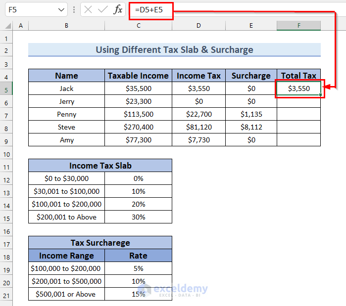
- Drag the Fill Handle down to get the Total Tax for every employee.
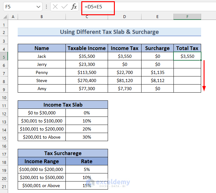
The results are as follows:
Read More: How to Calculate Sales Tax in Excel
Example 3 – Using Excel SUMPRODUCT Function
We can also calculate income tax on salary in Excel with the use of the SUMPRODUCT function.
Steps:
- Select the first row of the Income Tax Slab table.
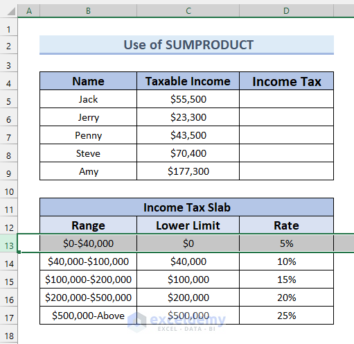
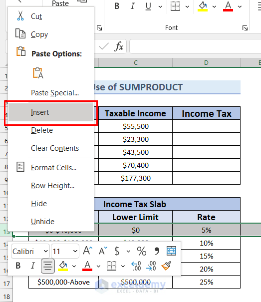
- Right-click on the row and select Insert to insert a new row.
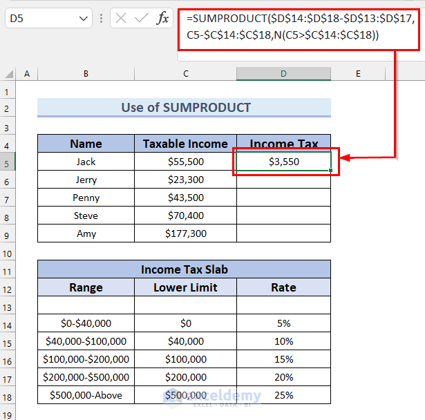
- In cell D5 enter the following formula:
=SUMPRODUCT($D$14:$D$18-$D$13:$D$17,C5-$C$14:$C$18,N(C5>$C$14:$C$18)) 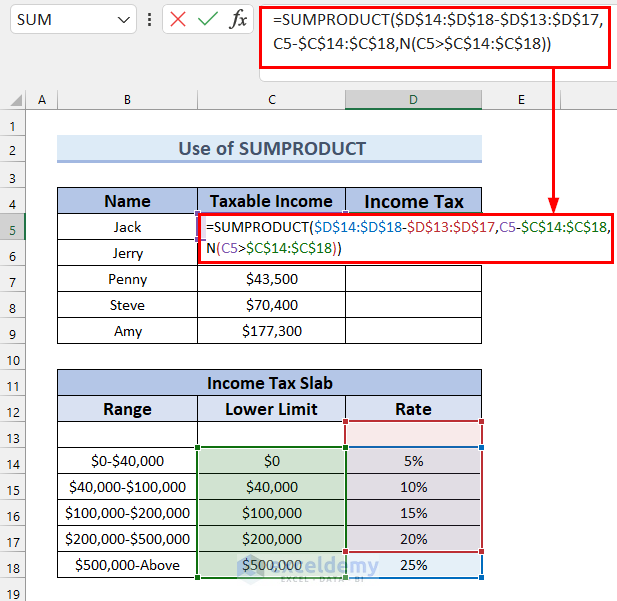
Here, in the SUMPRODUCT function, we select D14:D18-D13:D17 as array1 which figures out the differential rate. For array2 we select C5-C14:C18 where C5 is the Taxable Income for that specific employee and C5-C14:C18 returns the amount of each differential rate. And for array3 we use the N function which will return the value for C5>C14:C18 accordingly.
The SUMPRODUCT function will return the sum of the multiplied components of these 3 arrays.
In every case, we use absolute cell references so that the selected cell range remains fixed when using the AutoFill.
- Press ENTER to return the Income Tax for that specific employee.
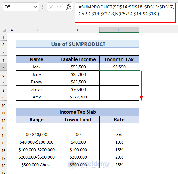
- Drag the Fill Handle down to copy the formula to the rest of the cells below.
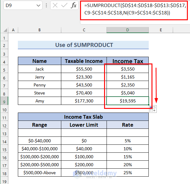
We have the Income Tax value for every employee.
Example 4 – Using VLOOKUP Function
To calculate income tax by using the VLOOKUP function, we add an extra column in the income tax slab, Cumulative, which represents the cumulative tax for that particular tax rate.
Steps:
- In cell D5, enter the following function:
=VLOOKUP(C5,$B$13:$E$17,4,TRUE)+(C5-VLOOKUP(C5,$B$13:$E$17,1,TRUE))*VLOOKUP(C5,$B$13:$E$17,3,TRUE) 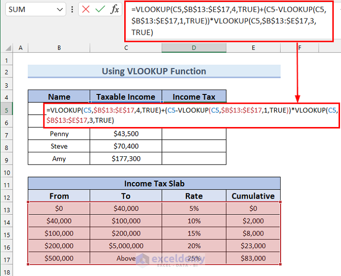
Formula Breakdown
- For the first VLOOKUP function, we select C5 as lookup_value, B13:E17 as table_array, 4 as col_index_number and for range_lookup we select TRUE. This will return the cumulative tax for C5.
- To get the income tax for C5 we use two more VLOOKUP functions. For the second VLOOKUP function, we select C5 as lookup_value, B13:E17 as table_array, 1 as col_index_number and for range_lookup we select TRUE.
- For the third VLOOKUP function, we select C5 as lookup_value, B13:E17 as table_array, 3 as col_index_number and for range_lookup we select TRUE.
- The second part of the formula will return the additional tax amount for C5. By adding these two parts, our formula will return the Income Tax value for C5.
- We use absolute cell references throughout, so that the selected cell range remains fixed when using the AutoFill.
- Press ENTER to return the Income Tax value for Jack.
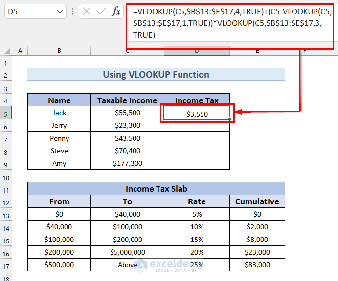
- Drag the Fill Handle down to get the Income Tax for every employee.
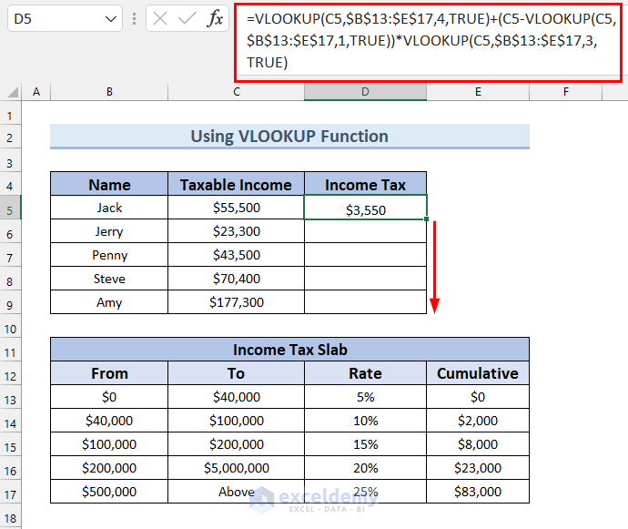
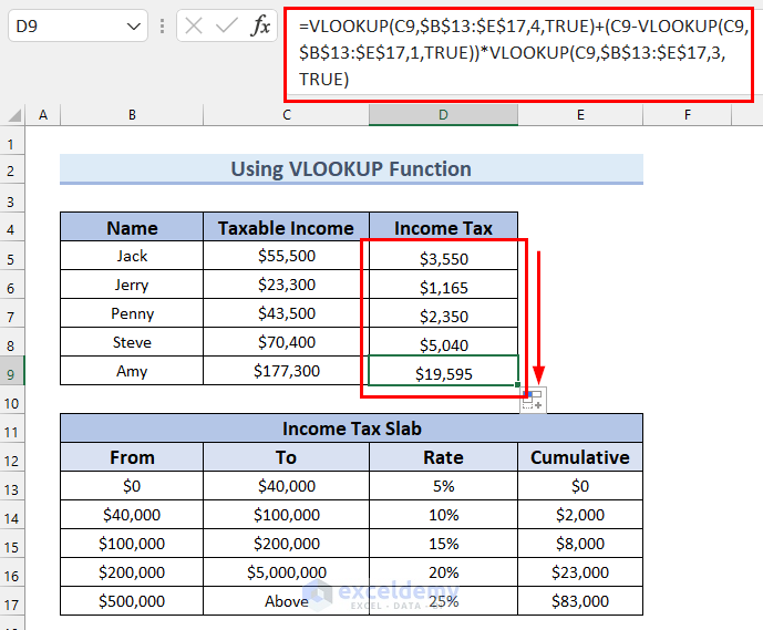
We have the Income Tax on salary for every employee.
Example 5 – Using Nested IF Function
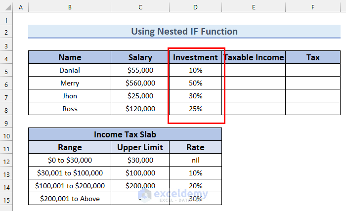
In this example we consider Investment. If someone has invested 30% or more than 30% of their salary, then the investment amount is deducted from the Salary to calculate Taxable Income.
Steps:
First we calculate the Taxable Income using the Investment rate and Salary.
- In cell E5 enter the following formula:
=IF(D5>=30%,C5-(C5*D5),C5) 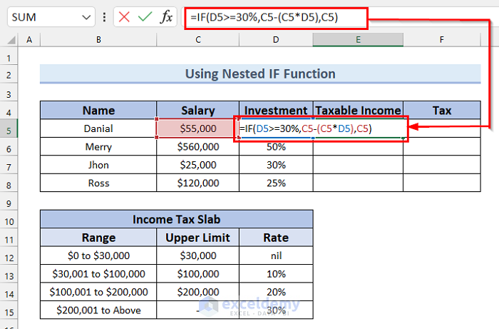
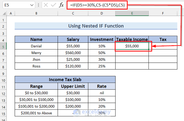
Here, D5>=30% is the logical_test, C5-(C5*D5) is the value_if_true, and C5 is the value_if_false. D5 is the investment rate, and C5 is the salary. If the logical test is TRUE the formula will deduct the Investment amount from the Salary and return the result as Taxable Income, and if the logical test is FALSE then it will return the Salary as Taxable Income.
- Press ENTER to return the Taxable Income for Danial.
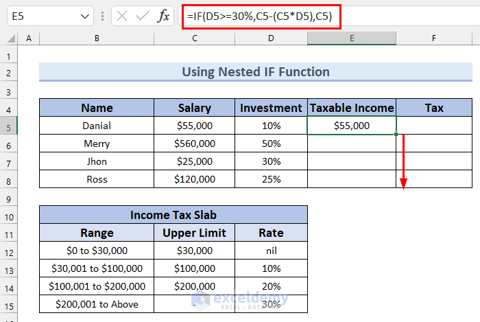
- Drag the Fill Handle down to get the Taxable Income for every employee.
The results are as follows:
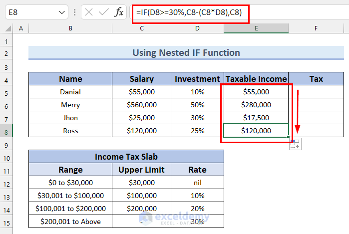
Now we can calculate Income Tax.
- In cell F5 enter the following formula:
=IF(E5<=$C$12,"nil",IF(E5<=$C$13,(E5-$C$12)*$D$13,IF(E5<=$C$14,(E5-$C$13)*$D$14+($C$13-$C$12)*$D$13,(E5-$C$14)*$D$15+($C$14-$C$13)*$D$14+($C$13-$C$12)*$D$13))) 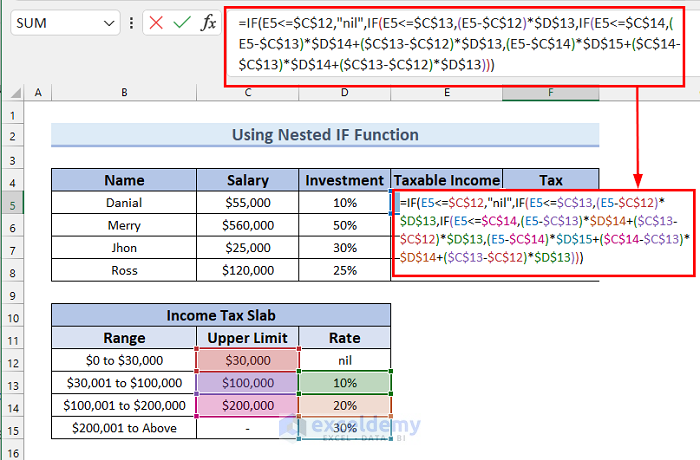
Formula Breakdown
- In this formula, for each logicat_test, we provide a value for value_if_true but for value_if_false we nest another IF function.
- If E5<=C12 then the formula will return the value “nil” and if not it will enter another logical test, which will check if E5<=C13. If it’s TRUE then it will return the value for (E5-C12)*D13 and if FALSE then it will go into another IF function, which will check if E5<=C14. If this logical_test is TRUE then it will return the value for (E5-C13)*D14+(C13-C12)*D13 and if the logical_test is FALSE then it will return the value of (E5-C14)*D15+(C14-C13)*D14+(C13-C12)*D13.
- Again, we use absolute cell references throughout so that the selected cell range remains fixed when using the AutoFill.
- Press ENTER to return the Tax for Danial.
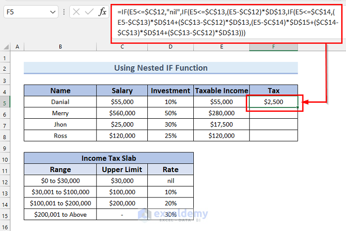
- Drag the Fill Handle down to get the Tax for every employee.
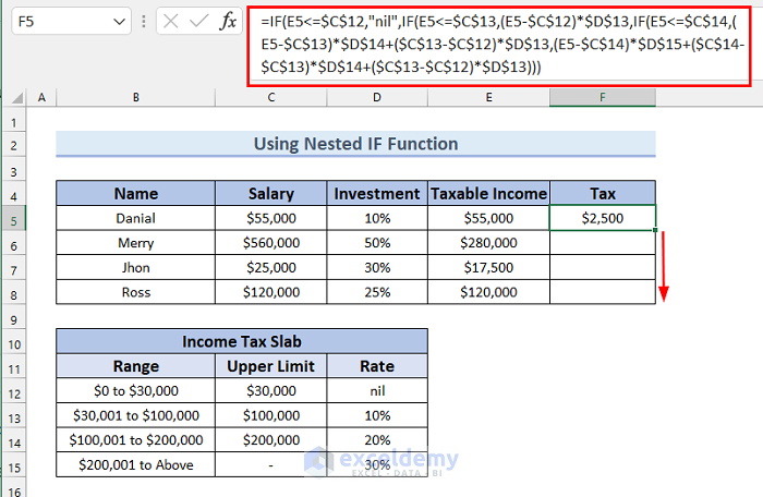
The results are as follows:
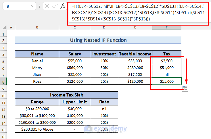
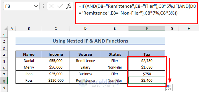
Example 6 – Using Nested IF & AND Functions with Payment Type
This example considers Payment Type and Status. If someone’s payment type is Remittance and status is Filer, then he/she will have to pay 5% tax on salary. If someone’s payment type is Remittance and status is Non-Filer, then he/she will have to pay 7% tax on salary. For all the other cases, a 3% tax on salary is applied.
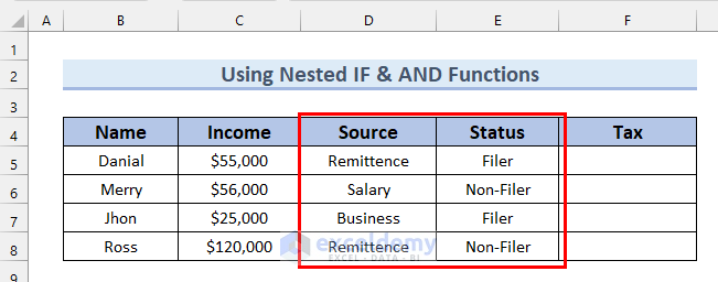
Steps:
- In cell F5, enter the following formula:
=IF(AND(D5="Remittence",E5="Filer"),C5*5%,IF(AND(D5="Remittence",E5="Non-Filer"),C5*7%,C5*3%)) 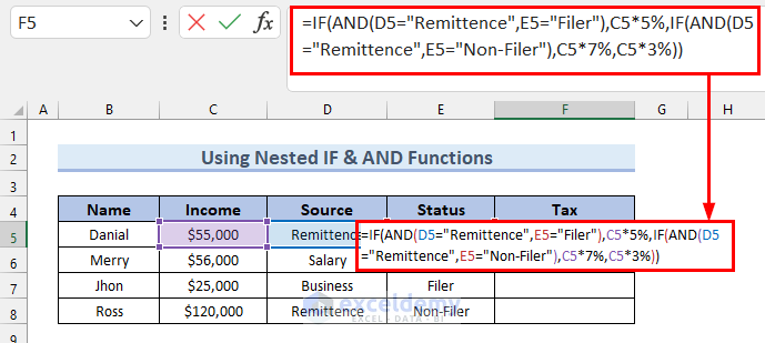
Formula Breakdown
- In the first IF function we use an AND function for the logical_test, C5*5% as value_if_true, and another IF function as value_if_false.
- In this second IF function we use another AND function as logical_test, C5*7% as value_if_true, and C5*3% as value_if_false.
- C5 is the Income. If the first AND is satisfied then the formula will return a 5% Tax on Income.
- If the second AND function is satisfied then the formula will return a 7% Tax on Income and for all the other cases the formula will return a 3% Tax on Income.
- In every case, we use absolute cell references so that the selected cell range remains fixed while using the AutoFill.
- Press ENTER to get the Tax amount for Danial.
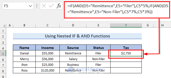
- Drag the Fill Handle to automatically copy the formula to all the cells in the column.
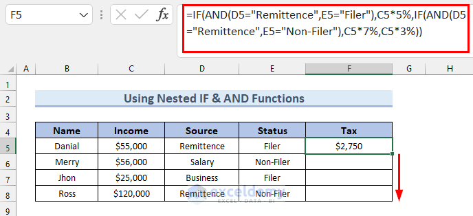
The Tax for all the employees is returned.
Download Practice Workbook
Related Articles
- How to Calculate Marginal Tax Rate in Excel
- How to Calculate Social Security Tax in Excel
- Formula for Calculating Withholding Tax in Excel
- How to Calculate Federal Tax Rate in Excel
<< Go Back to Excel Formulas for Finance | Excel for Finance | Learn Excel
Get FREE Advanced Excel Exercises with Solutions!

