How to Calculate IRR in Excel for Monthly Cash Flow: 4 Methods

Method 1 – Using IRR Function

Steps:

• Select a cell to put the IRR value in. We selected cell D19 for it.
• Write down the following formula in it.

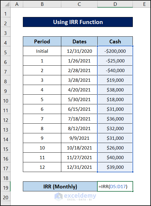
• Press Enter on your keyboard.

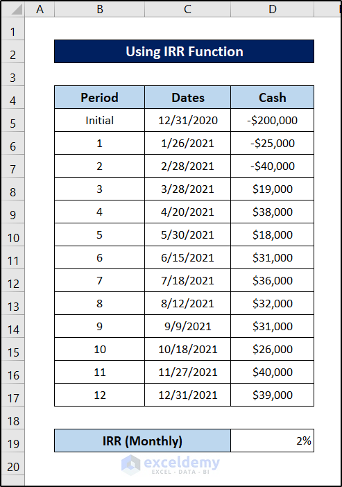
This will give you the IRR value on a monthly basis.

• Get the value on the yearly scale, follow the same procedure. Select the cell D20 and write down the following formula.

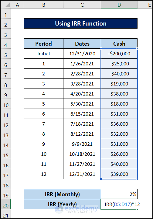
• Press Enter.

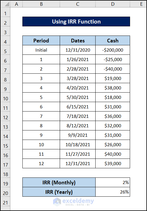
Calculate IRR using the IRR function for monthly cash flow in Excel.

Method 2 – Applying XIRR Function

Steps:

• Select a cell to put the IRR value in. Here, we have selected cell D19 for it.
• Write down the following formula.

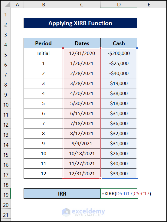
• Press Enter on your keyboard.

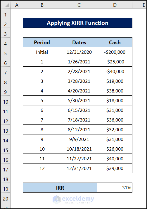
Calculate the IRR for monthly cash flow at irregular periods in Excel.

Method 3 – Utilizing MIRR Function

Steps:

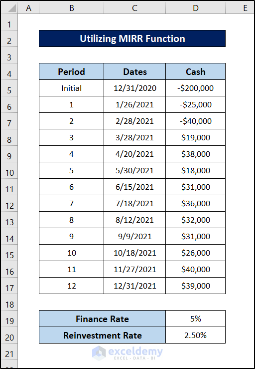
• Input the finance rate and the reinvest rate additionally for the dataset.

• Select a cell to store the IRR value. We have selected cell D21 here for this.
• Write down the following formula in it.

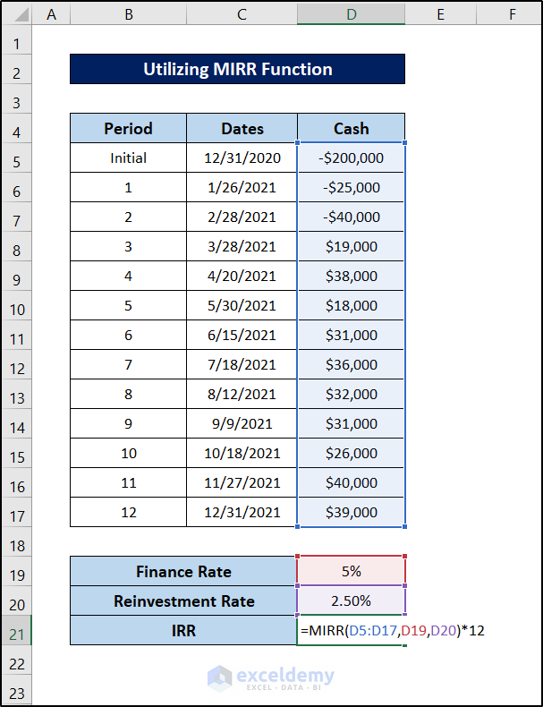
• Press Enter.

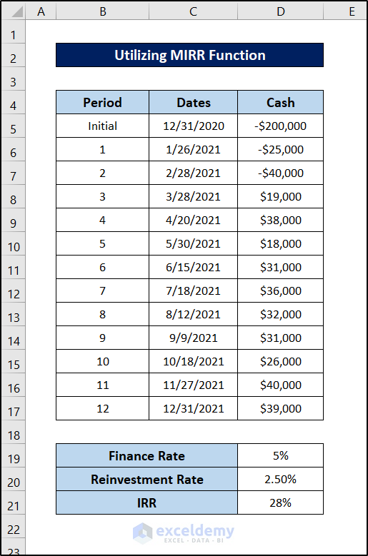
You will have the modified IRR in Excel for monthly cash flow.

Method 4 – Use of Conventional Formula

Steps to Prepare Dataset:

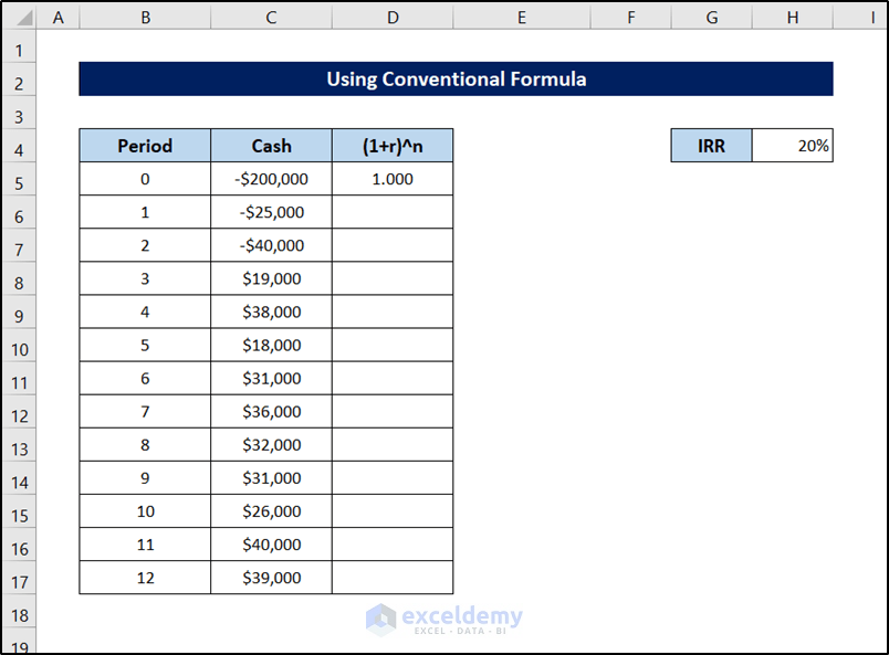
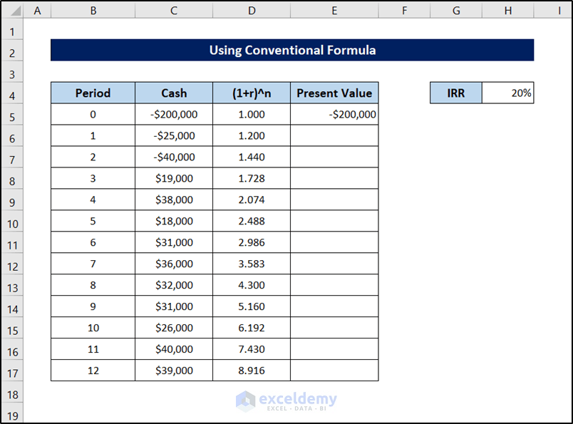
• An IRR at the start of the process. Let’s say 20%.
• Put it in a cell. Here we have put it in cell H4.

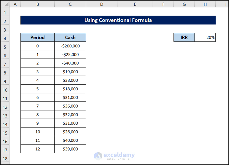
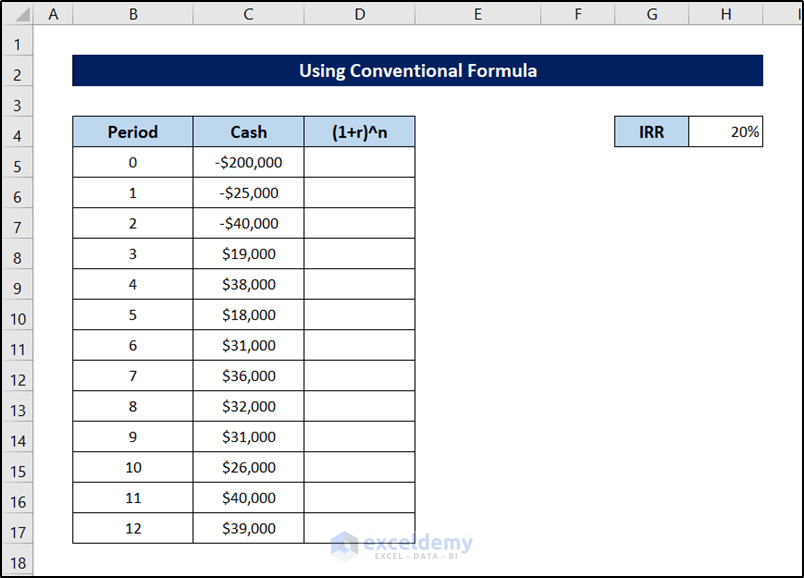
• Create a column to calculate the denominator of the NPV formula.

• Select cell D5 and write down the following formula.

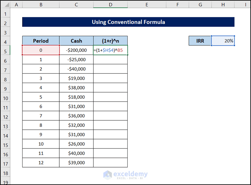
• Press Enter.

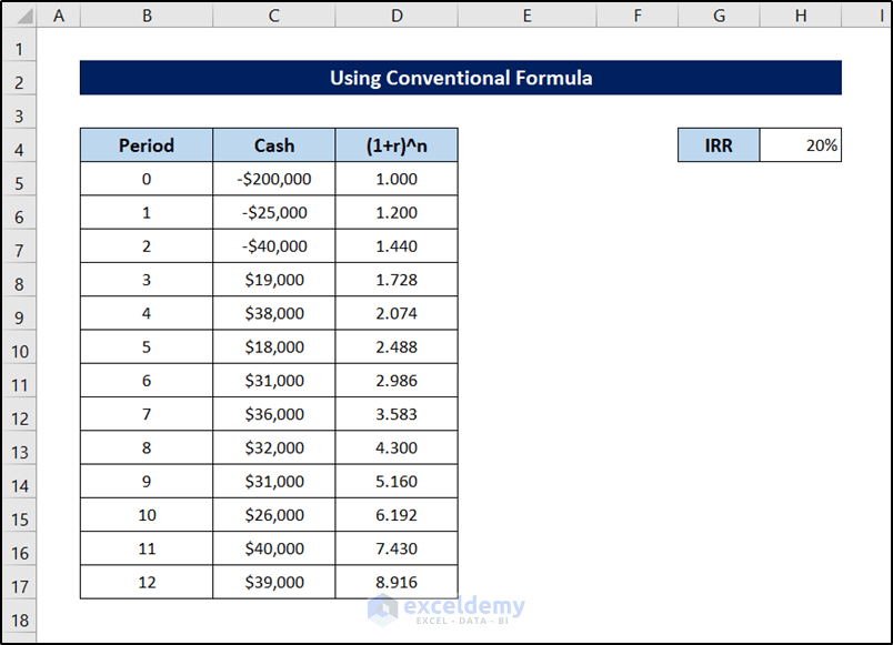
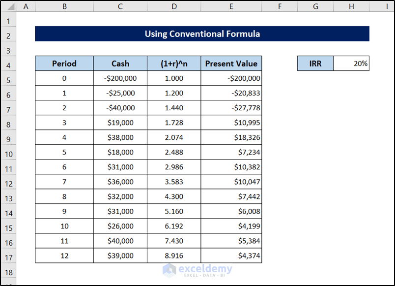
• Select the cell again. Now click and drag the fill handle icon to the end of the column to replicate the formula.

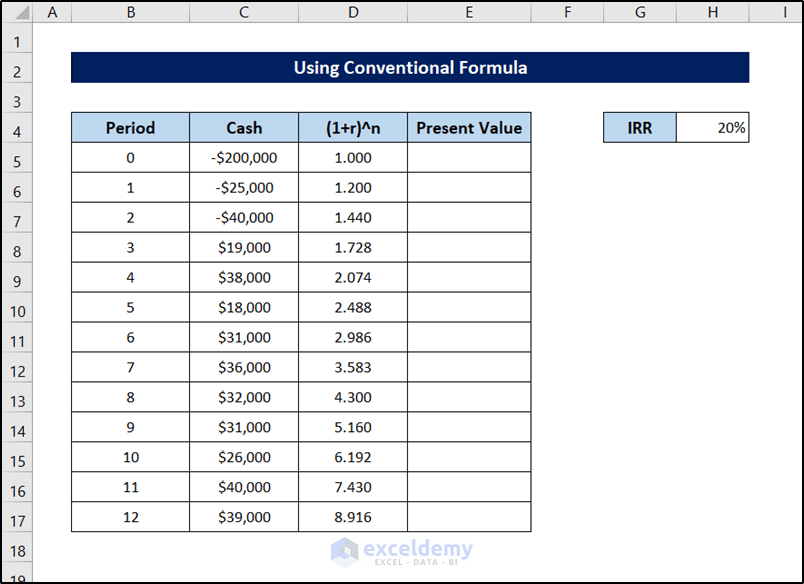
• Prepare a column for the present value of each payment.

• Select cell E5 and write down the following formula.

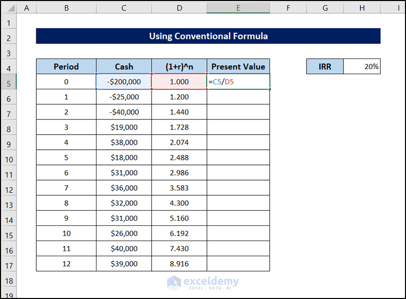
• Press Enter.

• Select the cell again and click and drag the fill handle icon to the end of the column to replicate the formula.

• Calculate the sum by selecting cell E18 and following the formula.

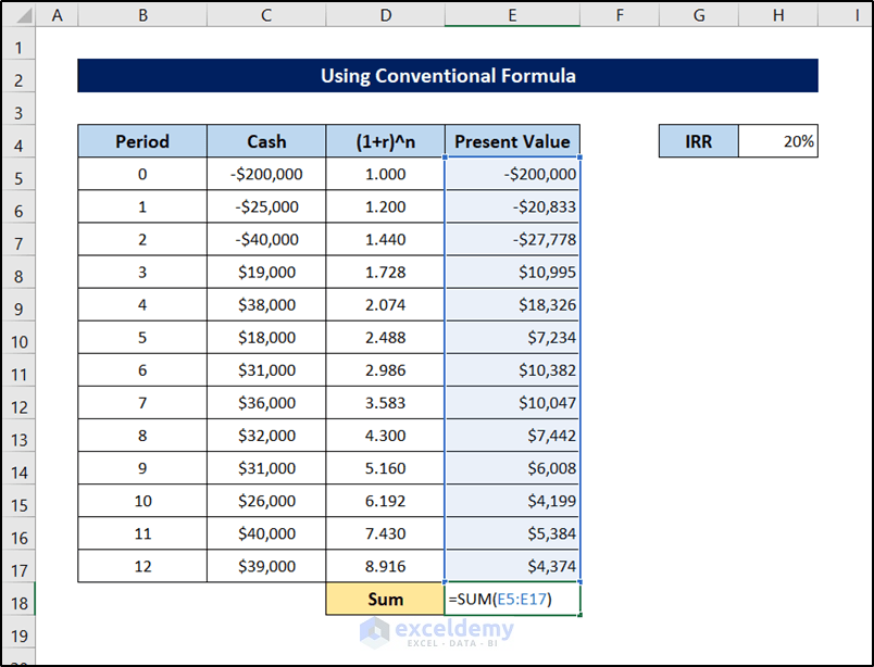
• Press Enter.

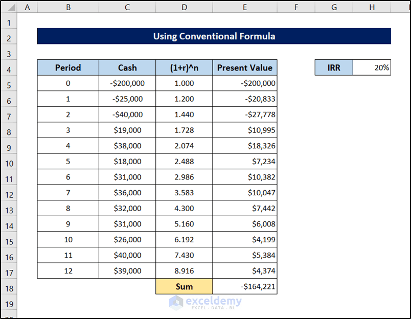
Steps to Calculate IRR Value:

The value of 20% IRR returns a net NPV of -164,221$, which is nowhere near the desired result. Keep changing the values of IRR that give the sum value at the lowest. We don’t have to repeat the same process as what we have done previously. Change the value in cell H4.

• Select cell H4 and change it to 10%.

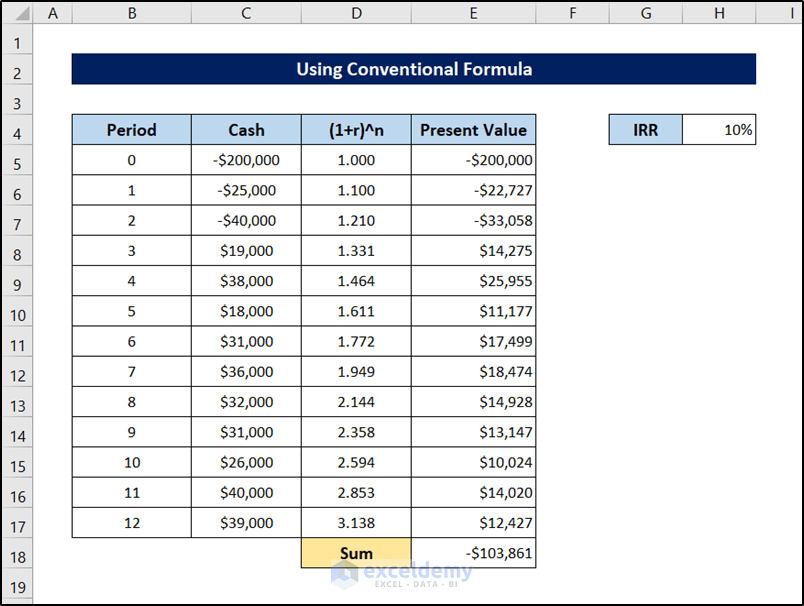
• The value in cell E18 has gone up and gotten closer to zero, which means it should go down.
• Enter a value of 5% in cell H4 and observe the changes.

• The value has further gone up. But not zero yet. Need to take a lower IRR value.
• Enter a value of 1% in cell H4.

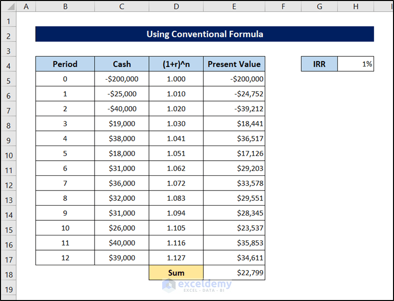
• The sum value is higher than zero now, which indicates that the IRR value should go up at this point.
• Putting the value of 2% in cell H4 now, we get something like this.

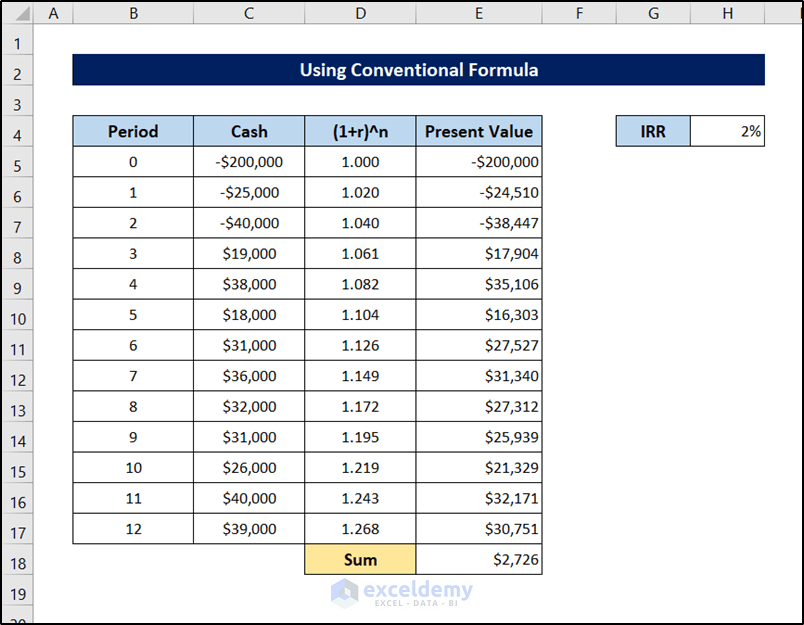
• Upon entering the value of 2.1%, the outcome looks like this.

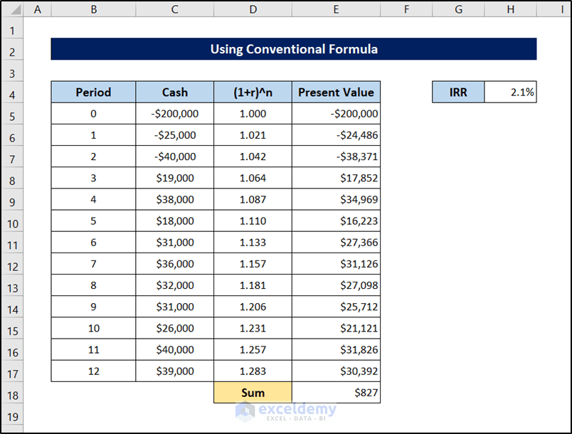
• With a value of 2.2%, it looks like this.

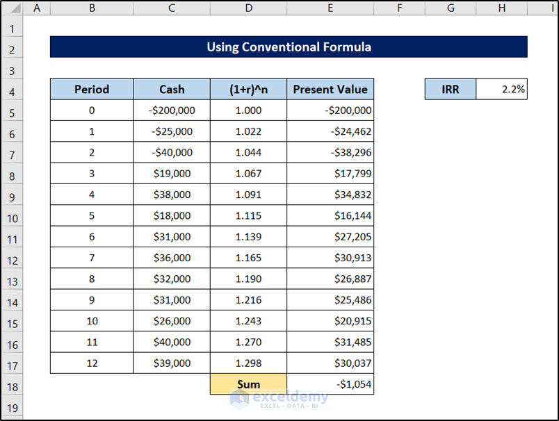
The value begins to deviate again, so we can conclude that 2.1% is the closest we can get to the IRR value for this range of data. This is also almost similar to the monthly IRR calculated with the IRR function in the first method.

Download Practice Workbook

You can download the workbook used for the demonstration from the link below. Download and try it yourself while you go through the article.

<< Go Back to Excel Functions | Learn Excel