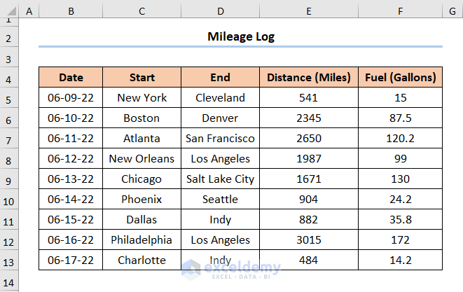
Throughout this article, we’re going to use the dataset shown below. The dataset consists of a mileage log with the Date of the journey, the Distance traveled (in Miles) between two Cities, and lastly, the volume of Fuel consumed (in US Gallons) to cover the Distance.
Step 1: Determine Mileage
- Insert an additional column for Mileage.
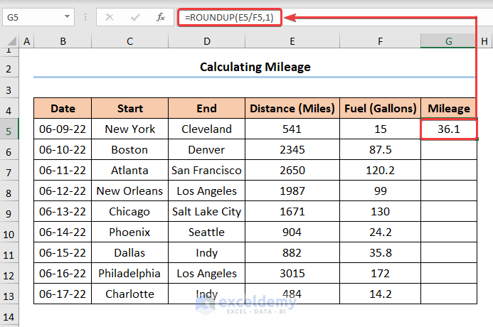
- Type in the ROUNDUP function to round up the result to one decimal place.
- Enter the following formula below:
=ROUNDUP(E5/F5,1)
In this expression, the E5 cell refers to the Distance (number argument) in miles while the F5 cell indicates the Fuel in US gallons (number argument). In contrast, the value of 1 refers to the num_digits argument, which rounds the result to the nearest 1 decimal place.
Step 2: Use the Fill Handle to Complete the Table
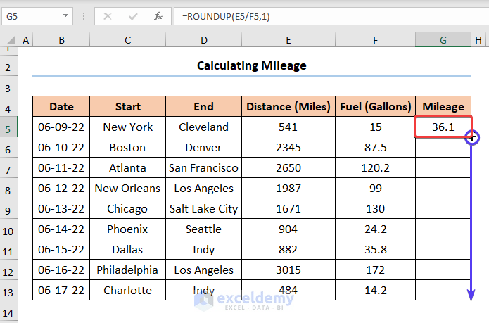
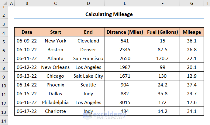
- Use the Fill Handle to copy the formula and fill out the table. The Mileage values are shown in the G5:G13 cells.
The results are shown below.
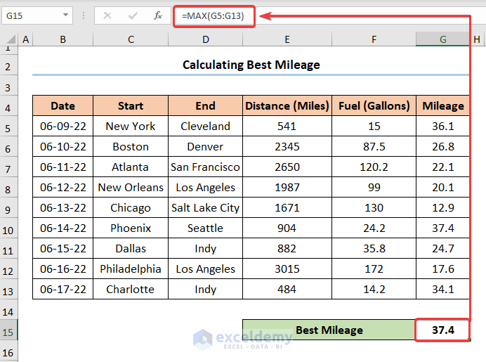
Calculating ‘Best Mileage’ in Excel
As we’ve discussed earlier, a bigger value of mileage is more desirable. Fortunately, Excel has the MAX function to determine the largest value from a selected range.
=MAX(G5:G13)
In this formula, the G5:G13 cells represent the Mileage (number1 argument).
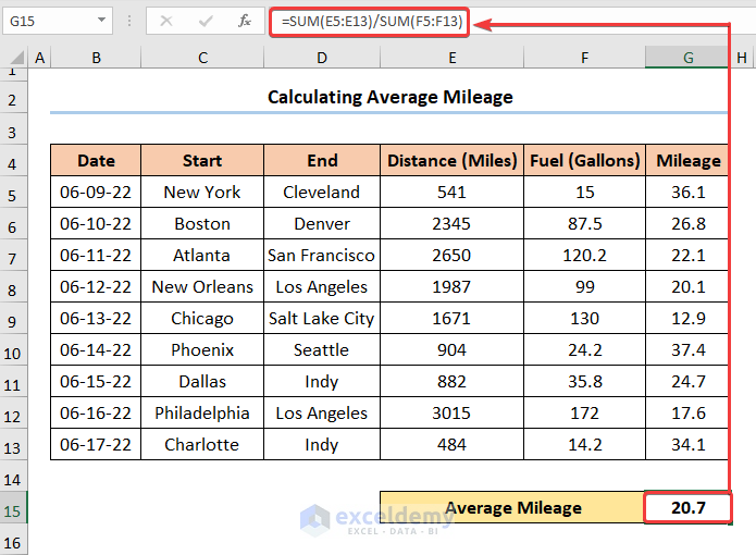
Computing Average Mileage
We can also determine the Average Mileage from the range using the SUM function, as shown in the formula below.
=SUM(E5:E13) / SUM(F5:F13)
In the above expression, the E5:E13 cells refer to the array range of the Distances, while F5:F13 cells represent the range of Fuel.
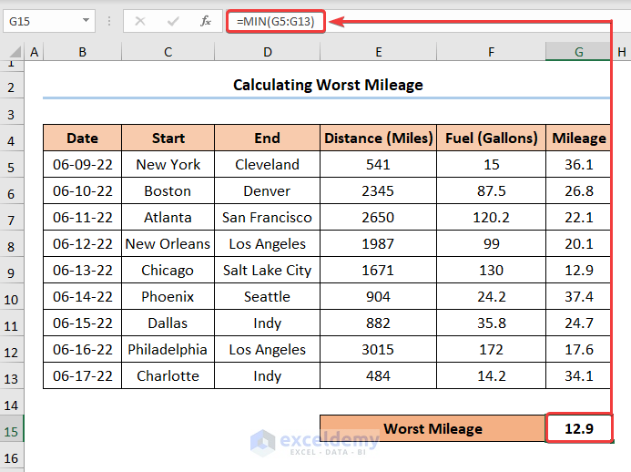
Determining Worst Mileage
=MIN(G5:G13)
In this formula, the G5:G13 cells represent the Mileage (number1 argument).
Download the Practice Workbook
You can download the practice workbook from the link below.
<< Go Back to Distance | Formula List | Learn Excel
Get FREE Advanced Excel Exercises with Solutions!

