How to Calculate Present Value of Future Cash Flows: 4 Methods

Method 1 – Use of PV Function to Calculate Present Value of Future Cash Flows

Steps:

Select a different cell, D6, where you want to calculate the present value.
Use the corresponding formula in the D6 cell.

=PV($C$4,B6,0,C6)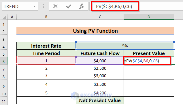

Formula Breakdown

The PV function will return the present value of an investment.

C4 denotes rate as the annual interest rate. The Dollar ($) sign denotes that the value of the C4 cell is fixed.
B6 denotes NPER as the total period of time.
As there is no Payment, so PMT will be 0.
C6 denotes FV as the Future Cash Flow.

Press ENTER to get the Present Value.

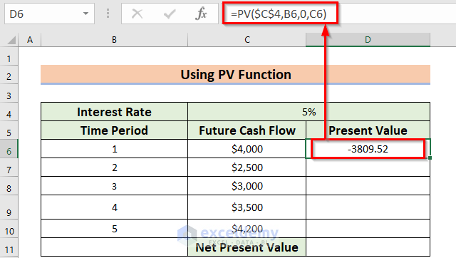
How to Calculate Present Value of Future Cash Flows

The Minus sign denotes that you must keep this amount at any monetary institute.

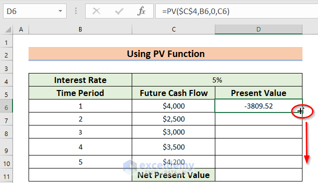
You must drag the Fill Handle icon to AutoFill the corresponding data in the rest of the cells D7:D10.

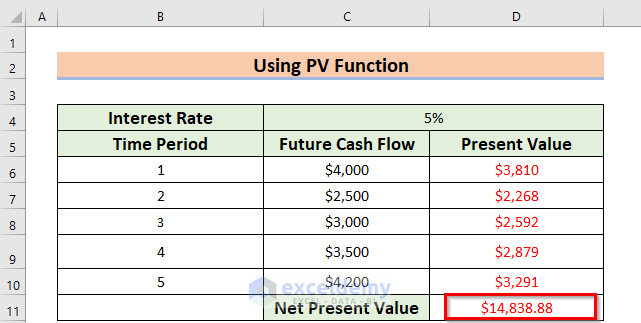
At this time, you will see the following result.

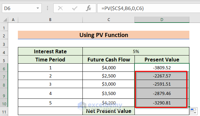
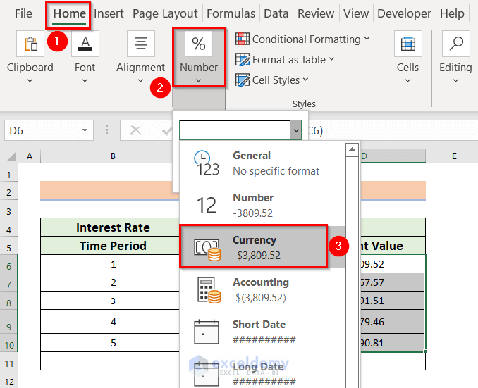
How to Calculate Present Value of Future Cash Flows

Select the data range. Here, I have selected D5:D10.
From the Home tab >> you should go to the Number feature.
In the Number feature >> Click the Drop-Down Arrow >> Choose currency.

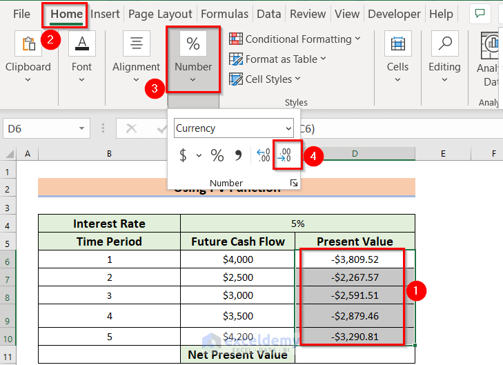
From the Number feature >> you need to Click two times on decrease decimal to decrease the decimal.

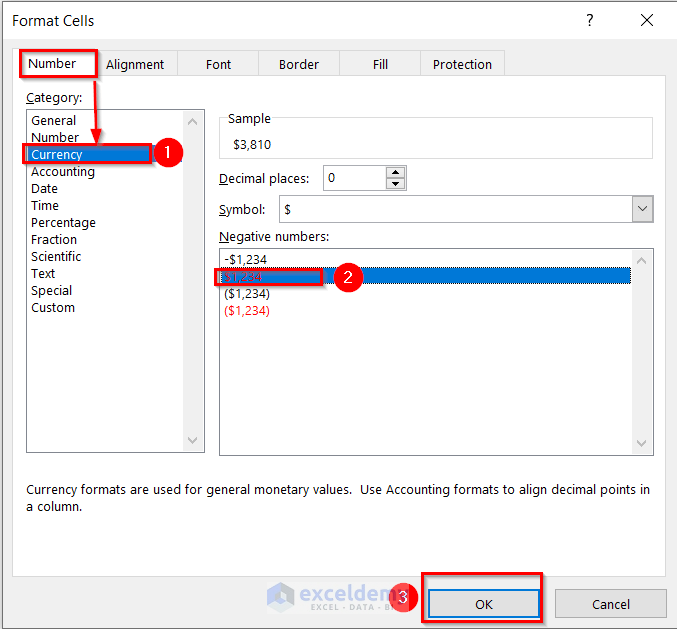
How to Calculate Present Value of Future Cash Flows

Press the CTRL+1 keys to open the Format Cells dialog box directly.

Use the Context Menu Bar or the Custom Ribbon to go to the Format Cells command.

Select the data range >> right-click on the data >> choose the Format Cells option.

In the case of using Custom Ribbon,

Select the data range >> from the Home tab >> go to the Format feature >> choose the Format Cells command.

After that, a dialog box named Format Cells will appear.

From that dialog box, you have to make sure that you are on the Number command.
Go to the Currency option.
Choose the second option from the Negative numbers option.
Press OK.

Get the total Present value, I will use the SUM function.

Select a different cell, D11, where you want to calculate the total Present Value.
Use the corresponding formula in the D11 cell.

=SUM(D6:D10)

Press ENTER.

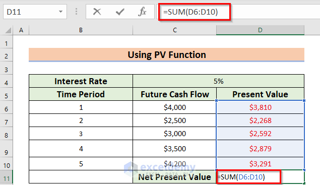
How to Calculate Present Value of Future Cash Flows

The SUM function will return the summation of the data range D6:D10. Get the following present value.

Method 2 – Applying NPV Function for Calculating Present Value

Steps:

Select a different cell, C11, where you want to calculate the present value.
Use the corresponding formula in the C11 cell.

=NPV(C4,C6:C10)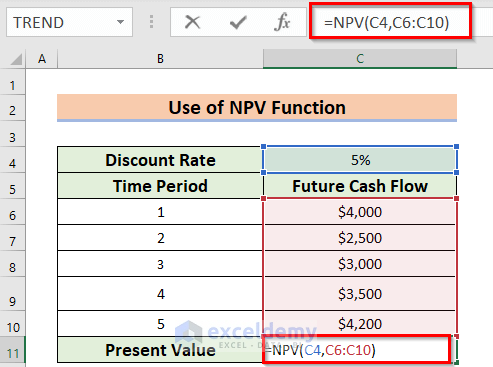

How to Calculate Present Value of Future Cash Flows

Formula Breakdown

The NPV function will return the net present value of an investment.

C4 denotes the discount rate. Which is 5%.
C6:C10 denotes the series of FV as the Future Cash Flows.

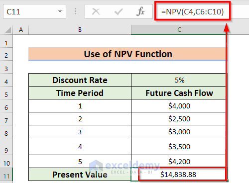
Press ENTER to get the Net Present Value.

Method 3 – Employing Generic Formula to Calculate Present Value of Future Cash Flows

Steps:

Select a different cell D6 where you want to calculate the Present Value.
Use the corresponding formula in the D6 cell.

=C6/((1+$C$4)^B6)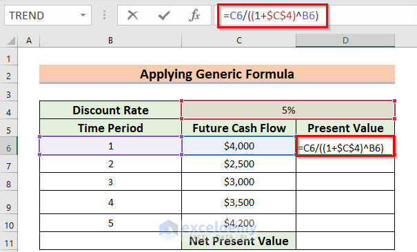

How to Calculate Present Value of Future Cash Flows

Formula Breakdown

C4 denotes the rate as the annual discount rate. The Dollar ($) sign denotes that the value of the C4 cell is fixed.
We added 1 with the discount rate.
- Output: 1.05.
The Power (^) sign raises it to a fixed power which is the value of B6 cell. That is the time period.
- Output: 1.05.
We divided the C6 cell value by 1.05.
- Output: $3,809.52.

Press ENTER to get the present value.

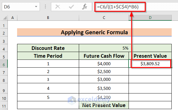
Drag the Fill Handle icon to AutoFill the corresponding data in the rest of the cells D7:D10.

Get the total present value, I will use the SUM function.

Select a different cell, D11, where you want to calculate the total present value.
Use the corresponding formula in the D11 cell.

=SUM(D6:D10)

Press ENTER.

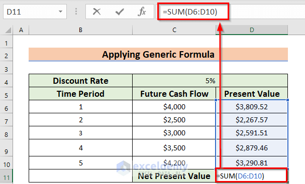
How to Calculate Present Value of Future Cash Flows

The SUM function will return the summation of the data range D6:D10. Lastly, you will get the following Present Value.

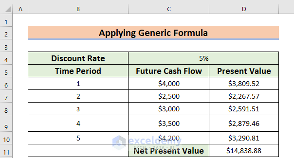
Method 4 – Using Generic Formula for Compound Interest

Steps:

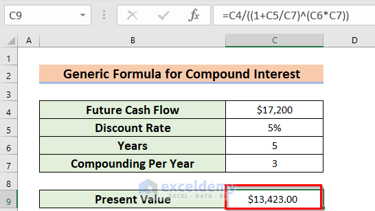
Select a different cell, C9, where you want to calculate the present value.
Use the corresponding formula in the C9 cell.

=C4/((1+C5/C7)^(C6*C7))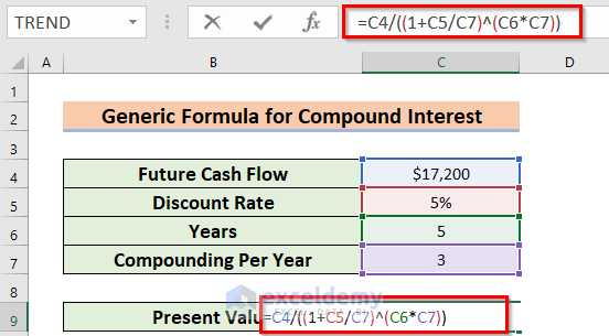

How to Calculate Present Value of Future Cash Flows

Formula Breakdown

C5 denotes rate as the annual discount rate.
We divided the cell value of C5 by Compounding year or C7 cell value.
- Output: 0.016666667.
We added 1 with the result.
- Output: 1.016666667.
We multiplied C6 with C7.
- Output: 15.
The Power (^) sign raises it to a fixed power.
- Output: 1.281382444.
We divided the C4 cell value by the output.
- Output:$13,423.00 .