Introduction to Tiered Commission
Sales representatives are motivated by commission rate tiers in a tiered commission system. Unlike flat compensation plans, tiered commission programs encourage sales representatives to meet sales targets. As a seller’s performance improves, their commission grows.
For example, let’s consider a scenario where sales representatives receive a 3% base commission on every deal until they sell a total revenue of $50,000.00 at the start of a new fiscal year. After reaching this threshold, their commission increases to 4% until they sell $100,000.00, and then further increases to 5%, and so on.
This payment structure aims to incentivize sales representatives to meet or exceed their quotas and keep closing transactions. The more sales representatives sell, the more money they earn.
Dataset Overview
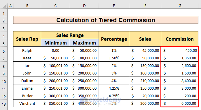
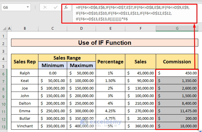
Suppose we have a large Excel worksheet containing information about several sales representatives from the Armani Group. The dataset includes the sales representatives’ names, sales ranges, percentage of tiered commission, and sales values (given in Columns B, C, E, and F, respectively).
Method 1 – Use the IF Function
Step 1
- Select a cell (e.g., G5) to apply the IF function.
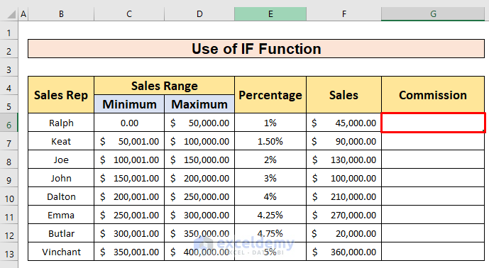
- Enter the following IF function:
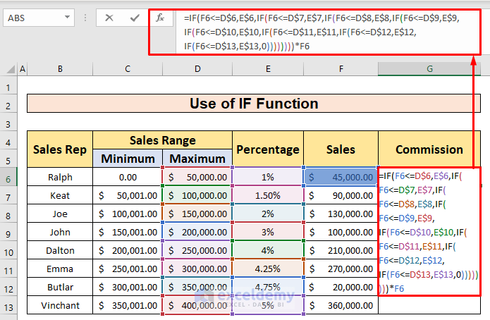
=IF(F6<=D$6,E$6,IF(F6<=D$7,E$7,IF(F6<=D$8,E$8,IF(F6<=D$9,E$9,IF(F6<=D$10,E$10,IF(F6<=D$11,E$11,IF(F6<=D$12,E$12,IF(F6<=D$13,E$13,0))))))))*F6Formula Breakdown
- The logical test checks if the sales value (F6) falls within the specified ranges (D$6 to D$13).
- The corresponding commission rate (E$6 to E$13) is applied.
- The final result is multiplied by the sales value (F6).
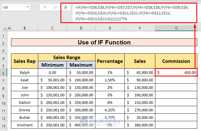
- Press Enter to get the tiered commission (e.g., $450.00).
Step 2
- AutoFill the IF function to other cells in column G.
Method 2 – Apply the VLOOKUP Function
Step 1
- Select a cell (e.g., D16) to apply the VLOOKUP function.
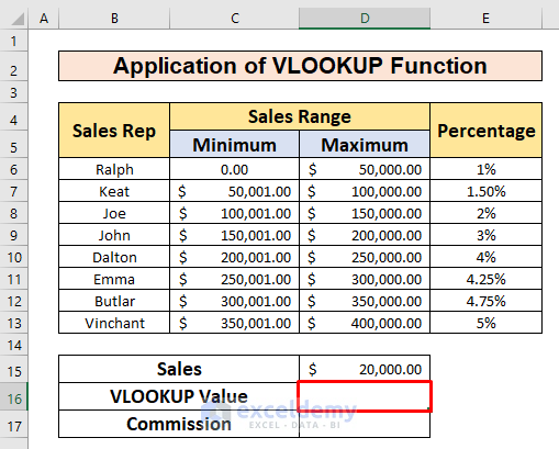
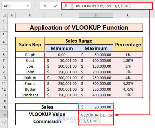
- Enter the following VLOOKUP function in the Formula bar:
=VLOOKUP(D15,C6:E13,3,TRUE)- D15 is the lookup value (sales target).
- C6:E13 is the table array containing sales ranges and commission rates.
- 3 represents the column index for the commission rate.
- TRUE enables approximate matching.
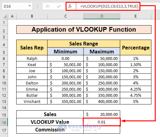
- Press Enter to get the commission rate (e.g., 0.01).
Step 2
- In cell D17, calculate the tiered commission:
=D15*D16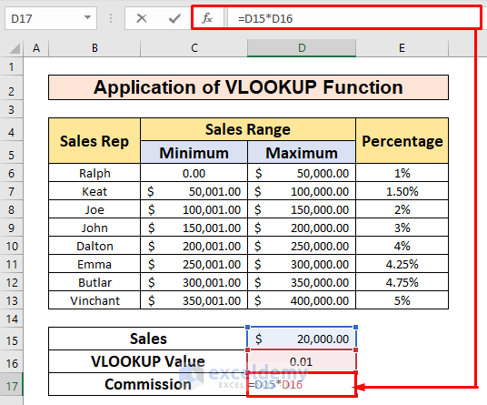
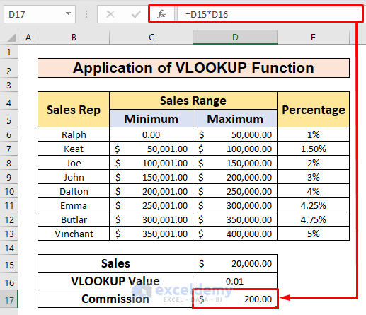
- Press Enter and you will get the tiered commission of $200.00.
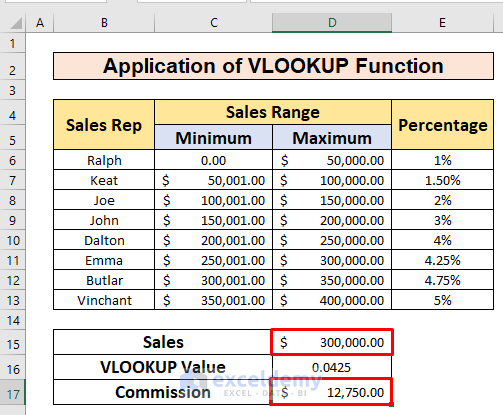
- You can verify the VLOOKUP function by changing the sales value (e.g., to $300,000.00) and observing the output.
Method 3 – Using SUMPRODUCT Function
Steps
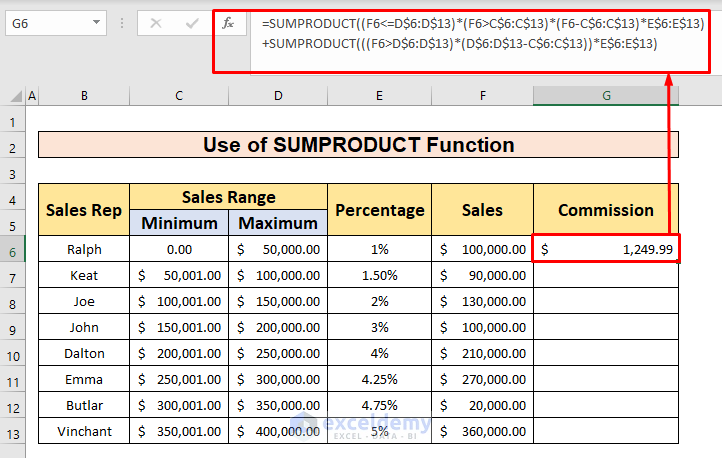
- Choose a cell (e.g., G5) where you want to calculate the tiered commission.
- Enter the following formula in the Formula bar:
=SUMPRODUCT((F6<=D$6:D$13)*(F6>C$6:C$13)*(F6-C$6:C$13)*E$6:E$13)+SUMPRODUCT(((F6>D$6:D$13)*(D$6:D$13-C$6:C$13))*E$6:E$13)-
- The formula combines conditions based on sales ranges and commission rates.
- It calculates the commission for each tier and sums them up.
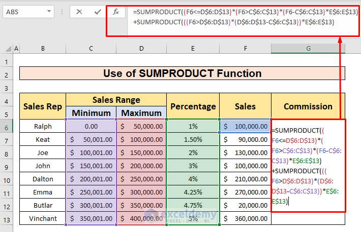
- Press Enter to get the tiered commission (e.g., $1,249.99).
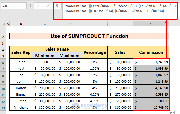
- AutoFill the SUMPRODUCT function to the remaining cells in column G.
Things to Remember
- #N/A! Error:
- Occurs when the formula or a function fails to find the referenced data.
- #DIV/0! Error:
- Happens when a value is divided by zero (0) or the cell reference is blank.
- #Value! Error (in Microsoft 365):
- Appears if you don’t select the proper dimension (e.g., matrix elements are not numbers).
Download Practice Workbook
You can download the practice workbook from here:
<< Go Back to Commission Bonus | Formula List | Learn Excel
Get FREE Advanced Excel Exercises with Solutions!

