Use the first two methods if you are only working with time. Use the second two methods if you are working with dates in Excel.
Method 1 – Calculate Turnaround Time Using TEXT Function in Excel
In the previous section, we had to change the format of the time difference to calculate the turnaround time as Excel automatically changes the time format
We can use the TEXT function to change the time format.
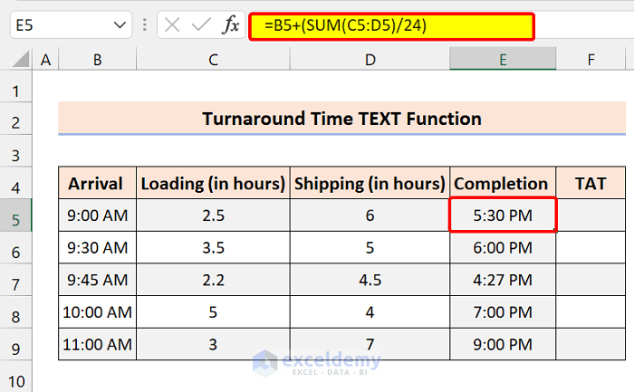
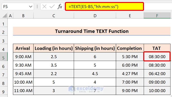
We have the following sample dataset of a company that loads products and ships them. You can see the arrival time of the product, loading time and shipping time. After completing all of these processes, the consumer gets the products.
To calculate the time needed for completion, we are adding the total hours to the arrival time.
The Generic Formula:
=arrival_time + (SUM(loading_time,shipping_time)/24)
We will calculate the turnaround time from this dataset.
The Generic Formula:
=TEXT(Completion Time – Arrival Time, Format)
The first argument is basic subtraction. In the format, you have to enter the time difference format that you want.
1.1 Display Turnaround Time in Hours
To calculate the turnaround time in hours, use the following formula:
=TEXT(E5-B5,"hh")
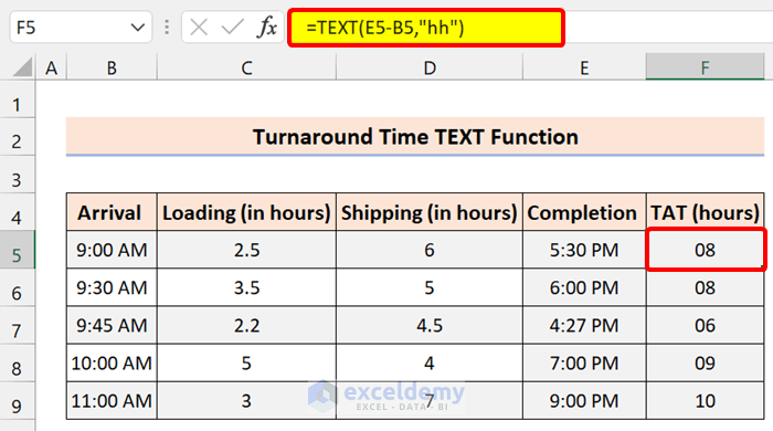
This formula will only deliver the outcome that displays the number of hours difference for turnaround time in Excel. If your outcome is 10 hours and 40 minutes, it will display 9 hours.
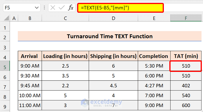
1.2 Display Only Minutes
To calculate turnaround time in only minutes worked, use the following formula:
=TEXT(E5-B5,"[mm]")
1.3 Display Only Seconds
To display turnaround time in just seconds format, use the following formula:
=TEXT(E5-B5,"[ss]")

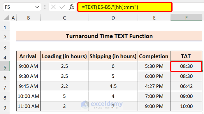
1.4 Display Hours and Minutes
If you want to calculate the turnaround time in hours and minutes format, use the following formula:
=TEXT(E5-B5,"[hh]:mm")
1.5 Display Hours, Minutes, and Seconds
For calculating turnaround time including all of these, use the following formula:
=TEXT(E5-B5,"hh:mm:ss")
We are using square brackets like [hh],[mm] or [ss] to give the whole number of Turnaround time in hours between the two dates, even if the hour is greater than 24. If you want to calculate the turnaround time between two date values where the distinction is more than 24 hours, utilizing [hh] will deliver the total number of hours for the turnaround time and “hh” will just give you the hours passed on the day of the end date.
Method 2 – Using MOD Function to Calculate Turnaround Time in Excel
If your time passes midnight, you will see the following turnaround time like the following:
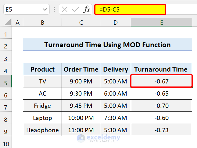
It will display a negative value. To resolve this problem, we can use the MOD function.
The Generic Formula:
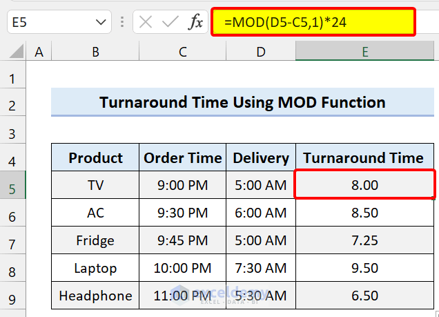
=MOD(Delivery-Order_time,1)*24 hrs
This formula handles the negative time by utilizing the MOD function to “reverse” negative values to positive values.
Select Cell E5 and enter the following formula:
=MOD(D5-C5,1)*24
Read More: How to Calculate Years of Service in Excel
Method 3 – Use of NETWORKDAYS Function to Calculate Turnaround Time
If you are working with dates to calculate the turnaround time, use the NETWORKDAYS function. In Microsoft Excel, the NETWORKDAYS function counts the number of dates between two specific dates.
The Generic Formula:
=NETWORKDAYS(start_date, completion_date)
Note to Remember: By default, the NETWORKDAYS function recognizes only Saturday and Sunday as weekends and you cannot customize these weekends. The NETWORKDAYS.INTL function will customize weekends.
To demonstrate, we are using this dataset:
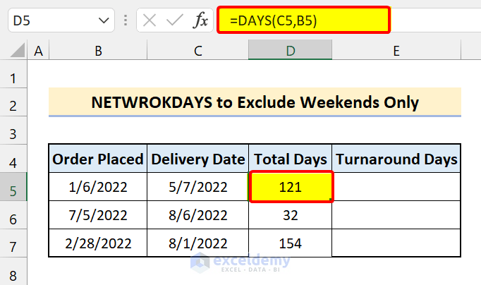
We have dates that indicate the dates of order placement and delivery date. We used the DAYS function to calculate the total days between the dates in the “Total Days” column. According to the formula, our turnaround days will be the difference between these dates. But, as the company has weekends, the NETWORKDAYS function won’t consider them.
3.1 Turnaround Time in Days
To calculate the turnaround time in days, select Cell E5 and enter the following formula:
=NETWORKDAYS(B5,C5)
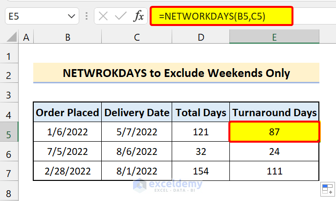
The turnaround time will be calculated.
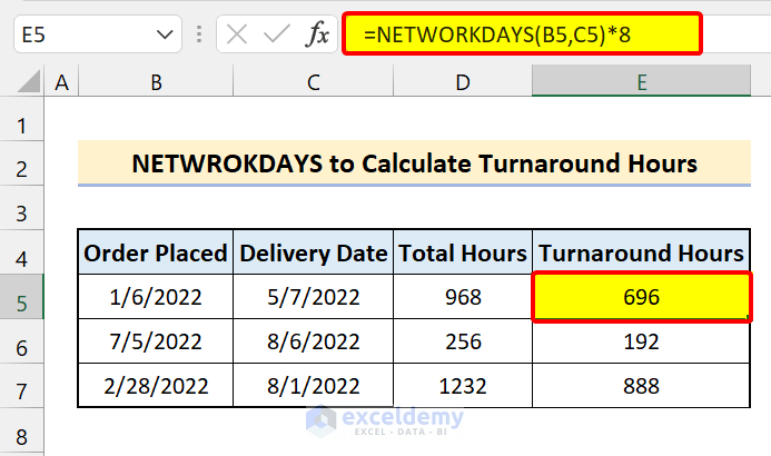
3.2 Turnaround Time in Hours
You can use this Excel formula to calculate the turnaround time in hours. You have to multiply the working hours with the function.
The Generic Formula:
=NETWORKDAYS(order date,delivery date)*working hours per day
To calculate the turnaround time in hours, select Cell E5 and enter the following formula:
=NETWORKDAYS(B5,C5)*8
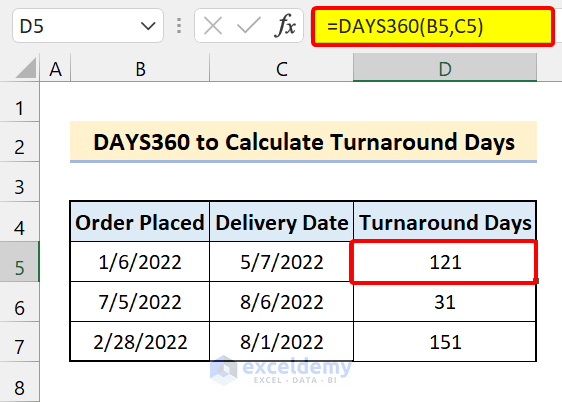
Method 4 – Use of DAYS360 Function to Calculate
If you don’t want to include the weekends or holidays in your around time, use the DAYS360 function.
The DAYS360 function calculates and returns the number of days between two dates based on a 360-day year (twelve 30-day months).
The Syntax:
=DAYS360(start_date,end_date,[method])
Arguments:
Start_date, end_date: These are the dates from where you want to know the difference. If your start_date happens after end_date, it will return a negative number. You should enter the dates in the DATE function or derive them from formulas or functions. For instance, use DATE(2022,2,22) to return on the 22nd day of February 2022. It will show some errors if you enter them as text.
Method: This is Optional. It is a logical value that determines whether to utilize the U.S. or European method in the analysis.
We will use the previous dataset for illustration.
To calculate the turnaround time in days, select Cell E5 and enter the following formula:
=DAYS360(B5,C5)
How to Calculate Turnaround Time in Excel Excluding Weekends and Holidays?
In the previous section, we used the NETWORKDAYS function to calculate the turnaround time in days or hours. This function doesn’t consider the weekends in the turnaround time. It automatically excludes the weekends.
The NETWORKDAYS function can be used to exclude the holidays in between the dates.
The Generic Formula:
=NETWORKDAYS(start_date, completion_date, holidays)
We can see in the sample dataset that there are some holidays.
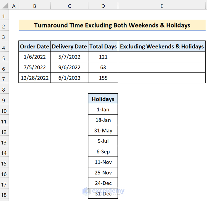
We will calculate the turnaround time excluding the weekends.
To calculate the turnaround time in days, select Cell E5 and enter the following formula:
=NETWORKDAYS(B5,C5,$D$10:$D$18)
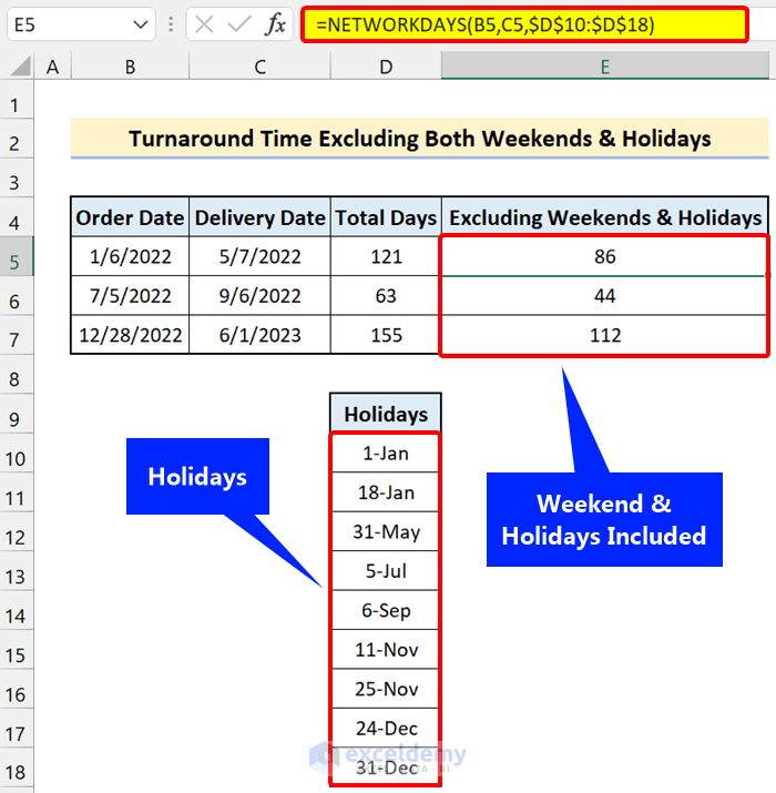
We have used absolute cell references for the range of cells containing holidays. It will give a wrong output if you don’t use absolute cell references because the cell references will change while auto-filling the cells in Column E.
Read More: How to Calculate Turnaround Time in Excel Excluding Weekends
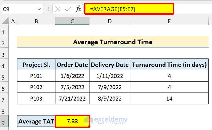
How to Calculate Average TAT in Excel?
Calculating the TAT (turnaround time) is equivalent to calculating the average time. You have to add all the turnaround time and divide them by the number of projects, days, weeks, etc.
We will use the AVERAGE function to calculate the average turnaround time.

We calculated the turnaround time for some projects. We used the NETWORKDAYS function to calculate the turnaround time in days excluding the weekends.
We used the following formula to calculate the turnaround time:
=NETWORKDAYS(C5,D5)
To calculate the average TAT in days, select Cell C9 and enter the following formula:
=AVERAGE(E5:E7)
Read More: How to Calculate Average Handling Time in Excel
How to Calculate TAT Percentage in Excel?
It will be an example of the increase in percentage for a particular turnaround time.
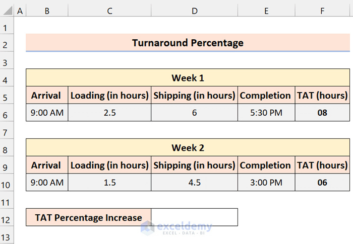
We have turnaround time of a company for two weeks. The company wants to improve its turnaround time. After they made a change, they reduced their loading and shipping time. This decreased their turnaround time.
To calculate the turnaround time in hours, we used the TEXT function in the formula:
=TEXT(E5-B5,"hh")
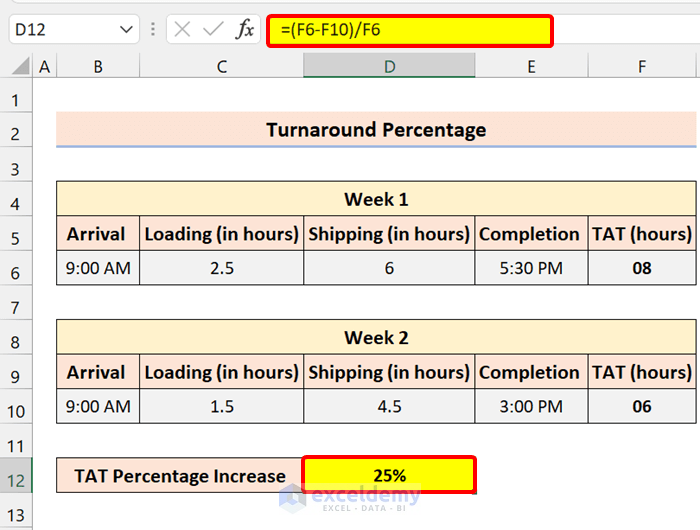
The Generic Formula to Calculate the TAT Percentage:
Increase in Percentage = (Week1 TAT – Week2 TAT) / Week1 TAT
To calculate the TAT percentage in days, select Cell D12 and enter the following formula:
=(F6-F10)/F6
Download Practice Workbook
Related Articles
- How to Calculate Elapsed Time in Excel
- How to Calculate Cycle Time in Excel
- How to Calculate Average Response Time in Excel
<< Go Back to Calculate Time | Date-Time in Excel | Learn Excel
Get FREE Advanced Excel Exercises with Solutions!
