Method 1 – Calculate YTD Average Using Excel AVERAGE Function
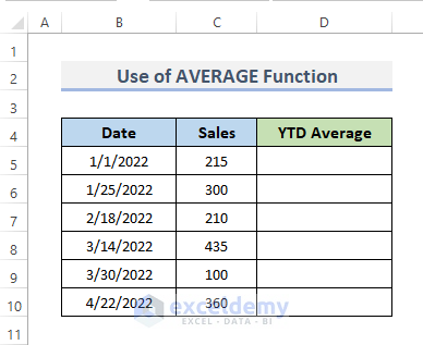
For calculating the year-to-date average, we are going to use the following dataset. The dataset contains some dates in column B, the total number of sales within those dates in column C and we want to calculate the average of year-to-date sales in column D.
STEPS:
- Select the cell where you want to put the formula to calculate the YTD average. For the sample, we selected cell D5.
- Enter the formula below into the selected cell.
=AVERAGE($C$5,C5)- Press Enter.
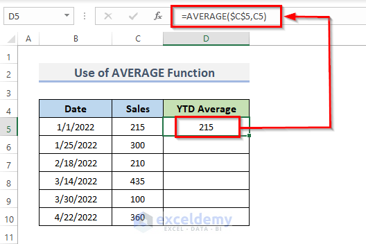
- It will output the YTD average.
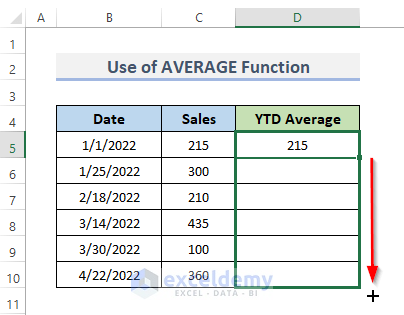
- To copy the formula over the range, drag the Fill Handle down. Or, double-click on the plus (+) sign to AutoFill the range.
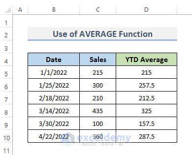
- It will output the average year-to-date sales in column D.
How Does the Formula Work?
The formula will calculate the YTD average, the dollar sign ($) refers to an absolute reference. By using the cell references as absolute reference $C$5 we just fixed the cell. This cell will be constant now as this is the first sale on those dates.
Read More: How to Calculate YTD (Year-to-Date) in Excel
Method 2 – Apply SUM Function to Calculate YTD Average
The sample dataset has dates in column B, the quantity of the sold product in column C, the total price for those products on that particular date in column D, and we want to calculate the YTD average of the products for the given dates in column E.
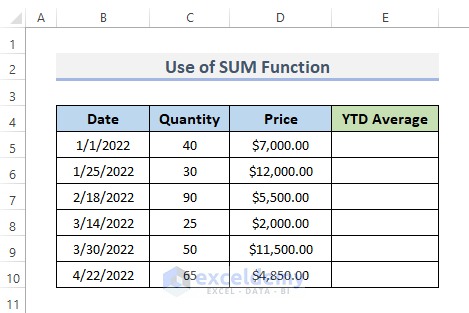
STEPS:
- Choose the cell (E5) where you want the YTD average formula.
- Add the formula below into the selected cell.
=SUM($D$5:D5)/SUM($C$5:C5)- Press Enter.
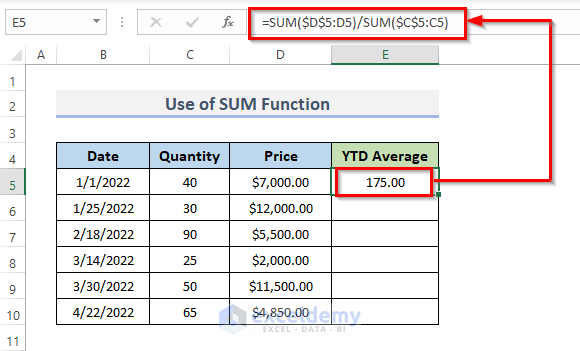
- It will output the YTD average.
- Drag the Fill Handle down or double-click on the plus (+) symbol to AutoFill the range.
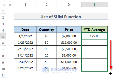
- Column E will be filled with the average year-to-date of the products for the given month.
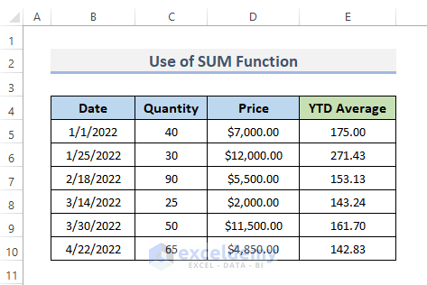
How Does the Formula Work?
The focus of this formula is the division between two consecutive values for price and quantity. The dividend of this equation is the sum of the product prices, whereas the divisor component is the sum of the product quantities using the SUM function.
Read More: How to Calculate MTD (Month to Date) in Excel
Method 3 – Use SUMPRODUCT Function to Calculate YTD Average in Excel
We will use the same dataset as in the second method.
STEPS:
- Add the formula below in cell E5.
=SUMPRODUCT($D$5:D5)/SUMPRODUCT($C$5:C5)- Press Enter.
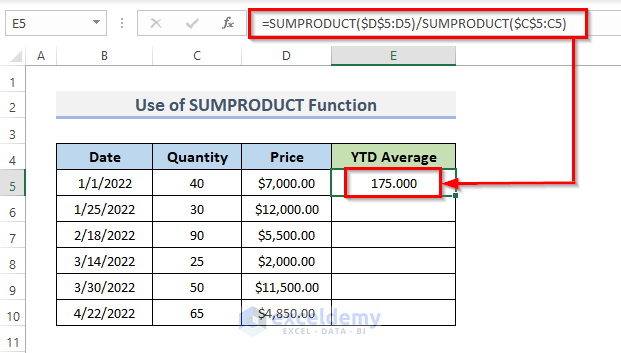
- It will output the YTD average.
- Drag the Fill Handle down or double-click on the plus (+) symbol to AutoFill the range.
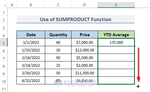
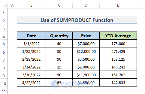
- Column E will show the average year-to-date.
Read More: How to Calculate YTD (Year to Date) in Excel
Method 4 – Merging SUM and COUNTIF Functions to Calculate YTD Average
The dataset has dates in column B, and the weekly income in column C, and in column D we will get the YTD average excluding zero values.
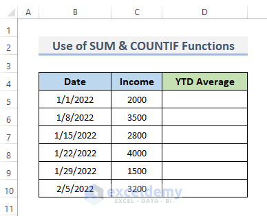
STEPS:
- Add the formula below in cell D5.
=SUM(C5:C10)/COUNTIF(C5:C10,"<>0")- Press Enter.
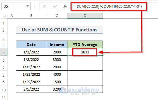
- It will output the YTD average.
- Drag the Fill Handle down or double-click on the plus (+) symbol to AutoFill the range.
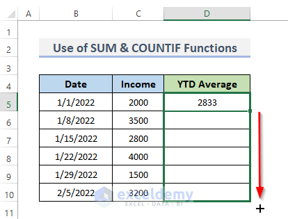
- Column D will display the average year-to-date.
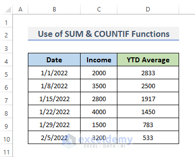
How Does the Formula Work?
The SUM function will sum the values in the range C5:C10. We divide the total sum for each cell value with the COUNTIF function, which will count the number of cells excluding zero values.
Read More: Excel Year to Date Sum Based on Month
Download Practice Workbook
<< Go Back to Excel Formulas for Finance|Excel for Finance|Learn Excel
Get FREE Advanced Excel Exercises with Solutions!

