In this article, we will demonstrate 6 ways to change semicolons to commas in Excel.
Suppose we have the dataset below containing some text delimited by semicolons.
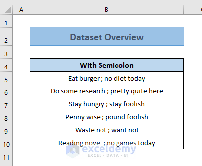
We can change the semicolons to commas manually, but this is not a practical and time-efficient approach, especially with large datasets. Instead, there are variety of Excel functions and features we can use.
Method 1 – Using the Find and Replace Command
The Find and Replace command finds characters or text within a provided range and optionally replaces these with specified characters or text.
Steps:
- Copy the data range which contains the semicolons to a new column and select this range.
- Press CTRL+H to open the Find and Replace dialog box.
- Type a semicolon (;) in the Find What field and put a comma (,) in the Replace with field.
- Click Replace All.
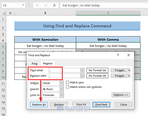
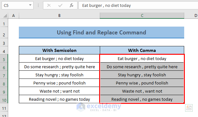
All the semicolons in the selected cells will be replaced with commas.
Method 2 – Using the SUBSTITUTE Function
The SUBSTITUTE function finds a text or character within a text string and replaces it with a new text or character.
Steps:
- Create a new column to put the modified text.
- Enter the following formula in the first cell of the new column:
=SUBSTITUTE(B5,";",",")
Here, B5 is the reference cell containing a semicolon.
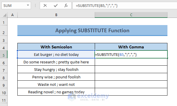
- Press ENTER to replace the semicolon with a comma.
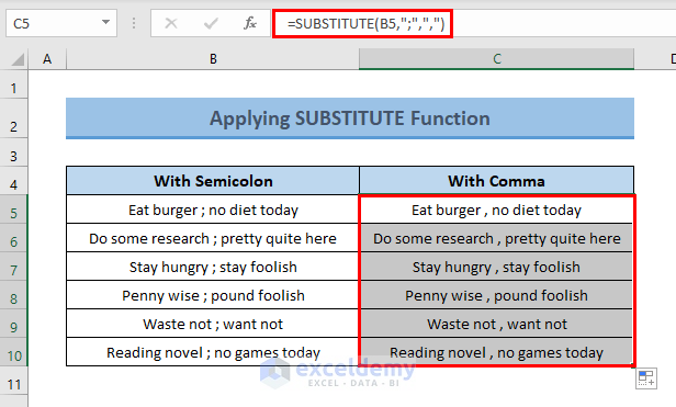
- Drag the Fill Handle tool down to Autofill the formula to the cells below.
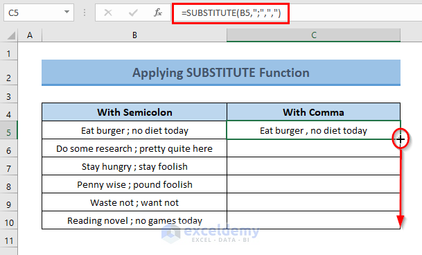
All the cells in the column have commas instead of semicolons.
Read More: How to Change Comma Style in Excel
Method 3 – Combining the CHAR and SUBSTITUTE Functions
The ASCII specification provides specific character codes from 1 to 255 for different characters. The CHAR function returns the corresponding character when a valid ASCII number is provided. We will use the CHAR function nested in the SUBSTITUTE function to change the semicolons to commas. The character code of the comma will be supplied in the CHAR function.
Steps:
- Select cell C5 and enter the following formula:
=SUBSTITUTE(B5,";",CHAR(44))
Here,
- B5 = The reference cell containing the semicolon.
- 44 = The character code for the comma.
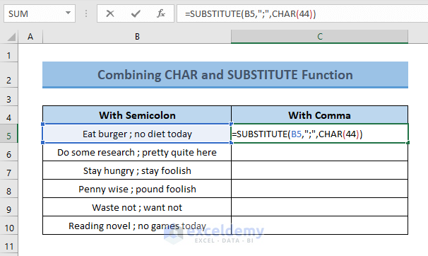
- Press ENTER and drag the formula down to replace all the semicolons with commas.
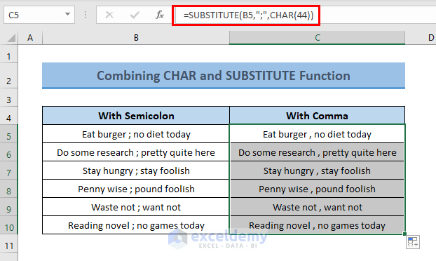
Formula Breakdown
44 is the character code of the comma, so, CHAR(44) returns a comma.
The SUBSTITUTE function replaces the semicolon (;) with the comma (,).
Method 4 – Using the REPLACE and SEARCH Functions
The REPLACE function is similar to the SUBSTITUTE function, but performs the replacement based on the starting number of the character in the text to be replaced, and the number of characters to be replaced. Nesting the SEARCH function in the REPLACE function will make the formula dynamic.
Steps:
- Select a cell where the replacement is required, apply the following formula, and drag it down to the rest of the cells below:
=REPLACE(B5,SEARCH(";",B5),1,",")
Here,
- B5 = The reference cell containing the semicolon.
- 1 = The number of characters to be replaced.
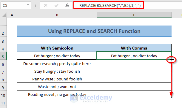
The semicolons are replaced with commas.
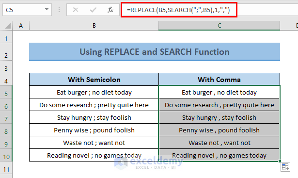
Formula Breakdown
SEARCH finds the semicolon (;) in cell B5 and returns its position.
Output => 12
REPLACE(B5,SEARCH(“;”,B5),1,”,”) = REPLACE(B5,12,1,”,”) replaces 1 character from the 12th position of the cell B5.
Final Output => Eat burger , no diet today
Method 5 – Combining Multiple Functions
Here, we will combine the CONCATENATE, LEFT, RIGHT, and SEARCH functions to perform the replacement.
Steps:
- Apply the following formula in cell C5:
=CONCATENATE(LEFT(B5,SEARCH(";",B5)-1)&","&RIGHT(B5,LEN(B5)-SEARCH(";",B5)))
Here, B5 = the reference cell containing a semicolon.
- Drag the formula to the cells below.
Formula Breakdown
- SEARCH(“;”,B5) finds the semicolon (;) in cell B5 and returns its position.
- Output => 12
- LEFT(B5,SEARCH(“;”,B5)-1) resolves to LEFT(B5,12-1) which resolves to LEFT(B5,11), which returns 11 characters from the left of the cell B5.
- Output => Eat burger
- The LEN function returns the number of characters in a text string. So, LEN(B5) returns 26.
- RIGHT(B5,LEN(B5)-SEARCH(“;”,B5)) resolves to RIGHT(B5,26-12) which resolves to RIGHT(B5,14), which returns 14 characters from the right side of the cell B5.
- Output => no diet today
- CONCATENATE(LEFT(B5,SEARCH(“;”,B5)-1)&”,”&RIGHT(B5,LEN(B5)-SEARCH(“;”,B5)))
resolves to CONCATENATE(Eat burger&”,”&no diet today), which returns the final output by concatenating “Eat burger” and “no diet today” with a comma between them.- Final Output => Eat burger , no diet today
Method 6 – Using the Text to Column Wizard and CONCATENATE Function
Finally, we will apply the Text to Column Wizard and CONCATENATE function together to perform the semicolon / comma replacement. The Text to Column Wizard will split the text separated by the semicolon into separate columns, then the CONCATENATE function will re-join the split strings using a comma delimiter.
Steps:
- Select the range of data.
- Go to the Data tab.
- Click the Text to Column feature from the Data Tools group.
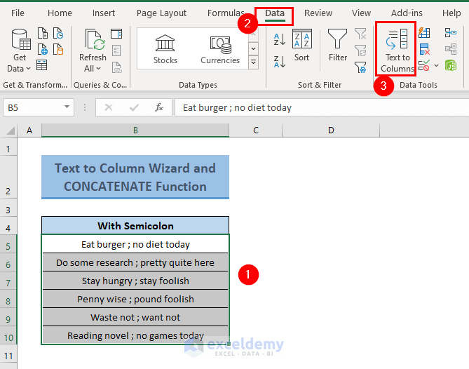
The Convert Text to Column Wizard (Step 1 of 3) box will appear.
- Keep the Delimited field marked (it is marked by default) and click Next.
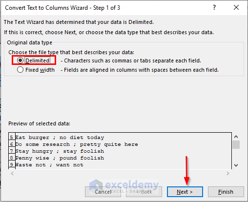
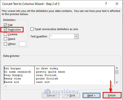
- In Step 2, mark the Semicolon field in the Delimiter section.
- Click Finish.
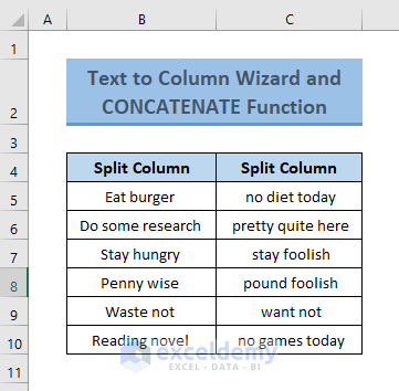
The strings are split into two columns, and the semicolons are gone.
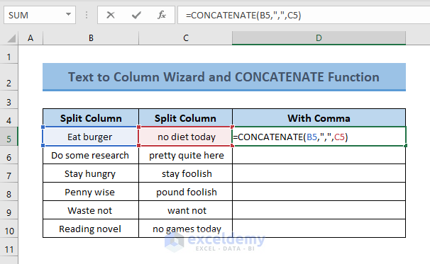
- Enter the following formula in an output cell:
=CONCATENATE(B5,",",C5)
Here,
- B5 = The first split cell.
- C5 = The second split cell.
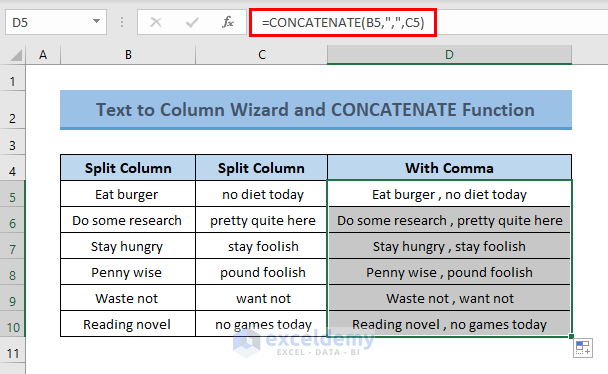
- Press ENTER and drag the formula down to concatenate all the cells with a comma.
Download Practice Workbook
Related Articles
- How to Convert Column to Row with Comma in Excel
- How to Change Comma in Excel to Indian Style
- [Fixed!] Style Comma Not Found in Excel
- How to Put Comma in Numbers in Excel
- How to Put Comma After 2 Digits in Excel
- How to Put Comma after 3 Digits in Excel
- How to Put Comma After 5 Digits in Excel
<< Go Back to How to Add Comma in Excel | Concatenate Excel | Learn Excel
Get FREE Advanced Excel Exercises with Solutions!

