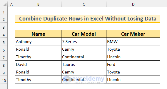
To demonstrate our methods to combine duplicate rows without losing data, we’ll use the following dataset:
Method 1 – Merging UNIQUE, IF & TEXTJOIN Functions
Steps:
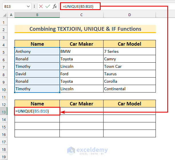
- Enter the following formula in cell B13.
=UNIQUE(B5:B10)The function will extract all the unique values from that range.
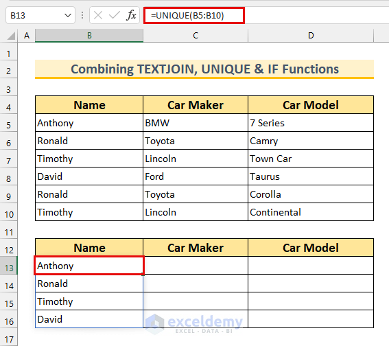
- Press ENTER.
Only the unique names are returned.
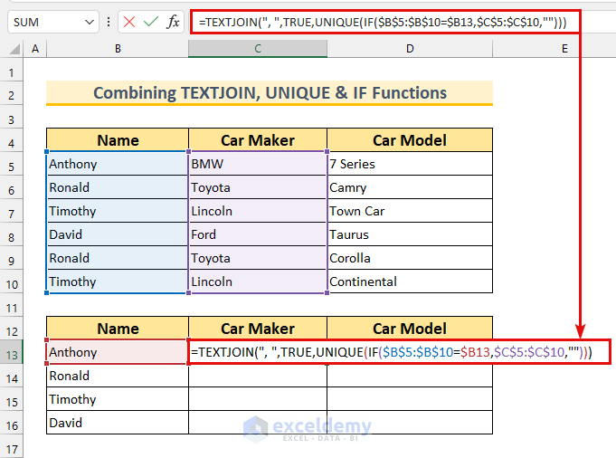
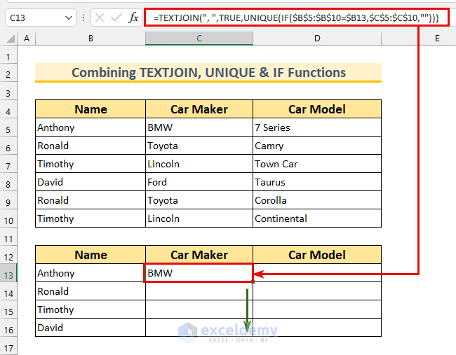
- Enter this formula in cell C13:
=TEXTJOIN(", ",TRUE,UNIQUE(IF($B$5:$B$10=$B13,$C$5:$C$10,"")))Formula Breakdown
- UNIQUE(IF($B$5:$B$10=$B13,$C$5:$C$10,””))
- Output: {“BMW”;””}.
- We check if the name from cell B13 is in the B5:B10 range.
- If there is a match, then the respective value from the C5:C10 range is extracted. Else, we’ll get a blank value.
- Only “BMW” matches our criteria.
- Our formula reduces to TEXTJOIN(“, “,TRUE,{“BMW”;””})
- Output: “BMW”.
- The TEXTJOIN function joins a range of strings into a single string.
- Our delimiter is a comma (“,”). Moreover, we’ve set ignore_empty as TRUE.
- Finally, we join the text “BMW” with nothing because we’re ignoring the empty value.
- Press ENTER.
- Use the Fill Handle to autofill the formula.
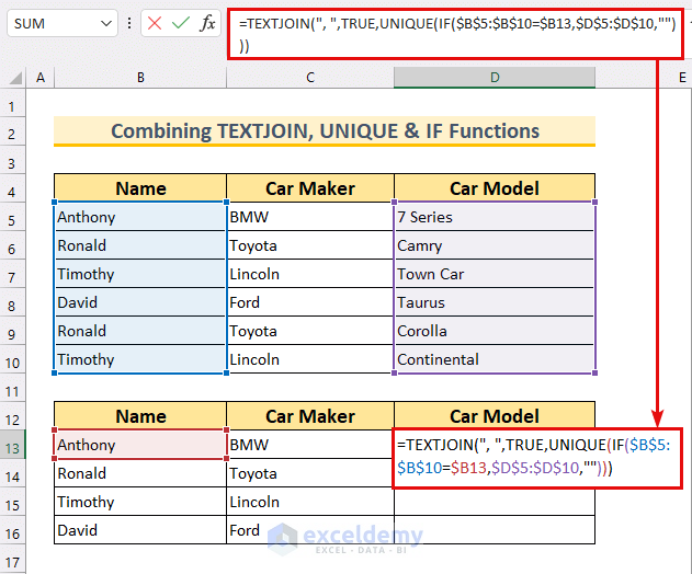
- Enter this formula in cell D13:
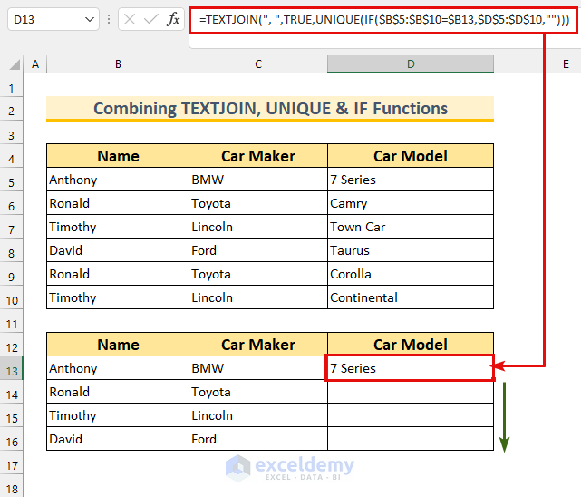
=TEXTJOIN(", ",TRUE,UNIQUE(IF($B$5:$B$10=$B13,$D$5:$D$10,"")))This formula is similar to the last formula.
- Press ENTER.
- AutoFill the formula.
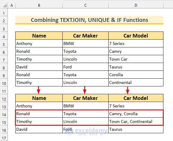
We’ve achieved our goal of combining duplicate rows without losing data.
Read More: How to Merge Duplicate Rows in Excel
Method 2 – Using 2 Helper Columns
Here we’ll use 2 helper columns, along with the CHAR & IF functions.
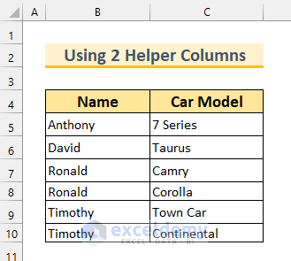
Steps:
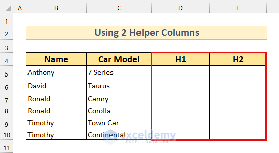
- Insert columns into the dataset as in the following image:
- Enter the following formula in cell D5:
=IF(B5=B4,C5&CHAR(10)&D4,C5)Formula Breakdown
- CHAR(10) returns a line break.
- We check if the value from the lower cell is the same as the upper cell.
- When it is the same, we join the values from “Car Model” with a line break, else we keep the cell value as it is.
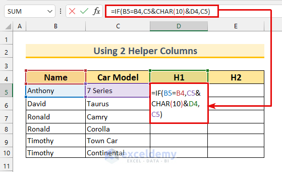
- Press ENTER.
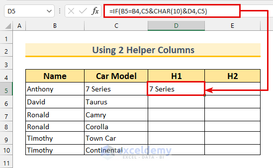
- AutoFill the formula.
- Enter the following formula in cell E5:
=IF(B6<>B5,"Combined Row","")Here we check if the value from cell B6 is not equal to the value from cell B5. If true, then we return “Combined Row”, else we’ll get a blank cell.
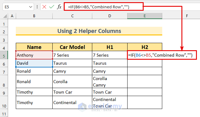
- Press ENTER and AutoFill the formula.
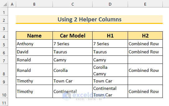
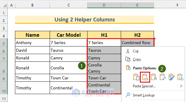
- Copy the values from the 2 helper columns and replace them using the “Paste as Values” option.
Now we remove the extra data.
- Delete the empty rows.
- Replace the values of column C with column D.
- Delete the columns that we created.
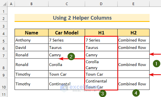
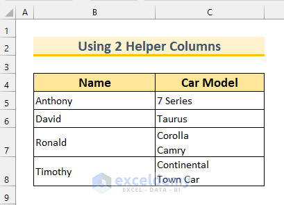
We’ve successfully combined duplicate rows without losing data.
Method 3 – Using a PivotTable
Steps:
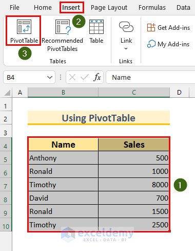
- Select the range B4:C10.
- From the Insert tab, select PivotTable.
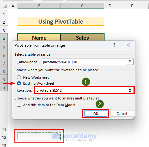
The “PivotTable from table or range” dialog box will appear.
- Select Existing Worksheet.
- Select B12 as the Location.
- Click on OK.
The “PivotTable Fields” dialog box will appear.
- Drag the “Name” field into Rows.
- Drag the “Sales” field into Values.
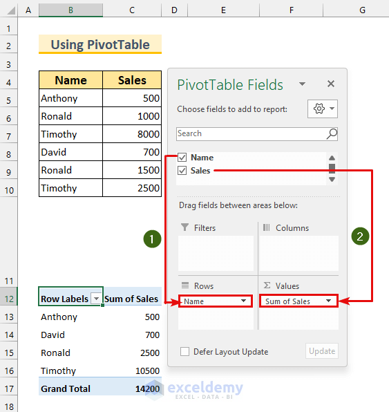
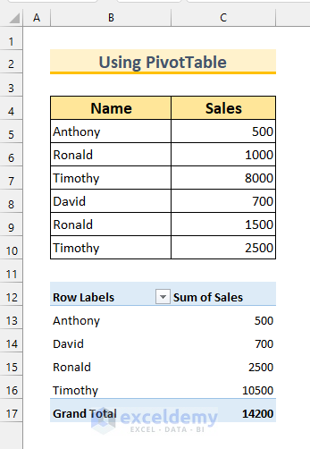
Duplicate rows have been combined without losing data.
Method 4 – Using Consolidate Feature
Steps:
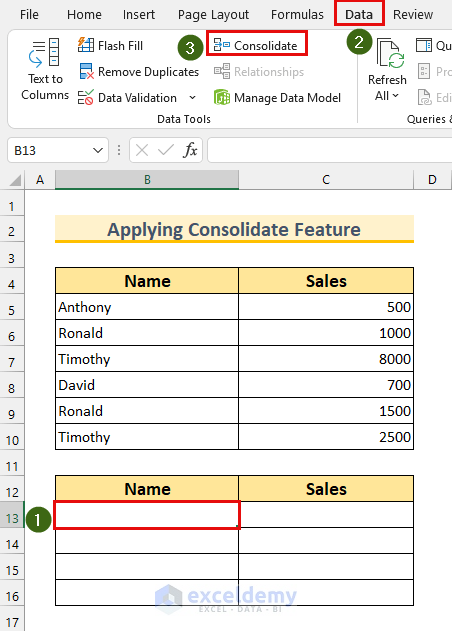
- Select cell B13. We’ll consolidate our data here.
- From the Data tab, select Consolidate.
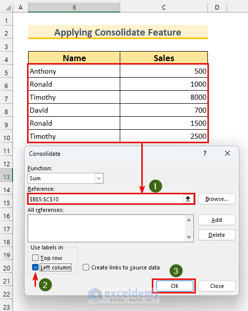
The Consolidate dialog box will appear.
- Select the cell range B5:C10 as “Reference:”.
- Select “Left column” from the “Use labels in” section.
- Click OK.
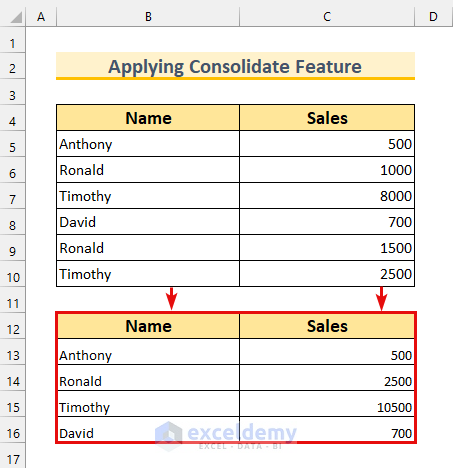
We’ve successfully combined duplicate rows without losing data.
Method 5 – Using Subtotal Feature
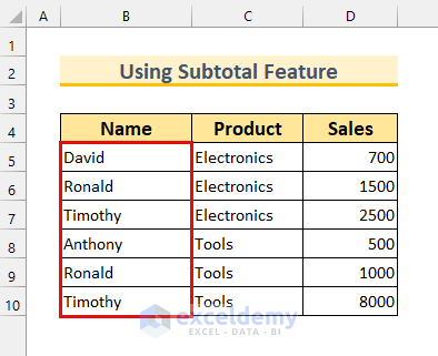
Here, we need to sort our data before applying the formula.
Steps:
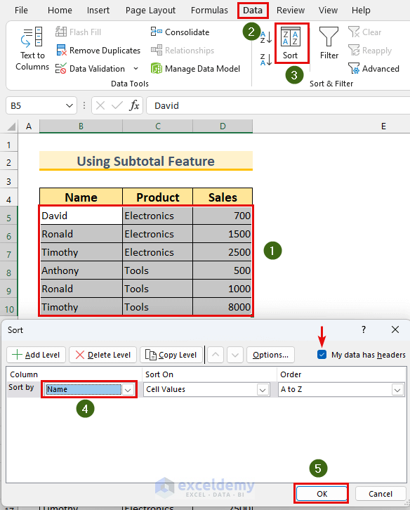
- Select the range B5:D10.
- From the Data tab, select Sort.
A Sort dialog box will appear.
- Make sure “My data has headers” is selected if you select range B4:D10.
- Select “Name” in the Sort by section.
- Click OK.
Now we can use the Subtotal feature.
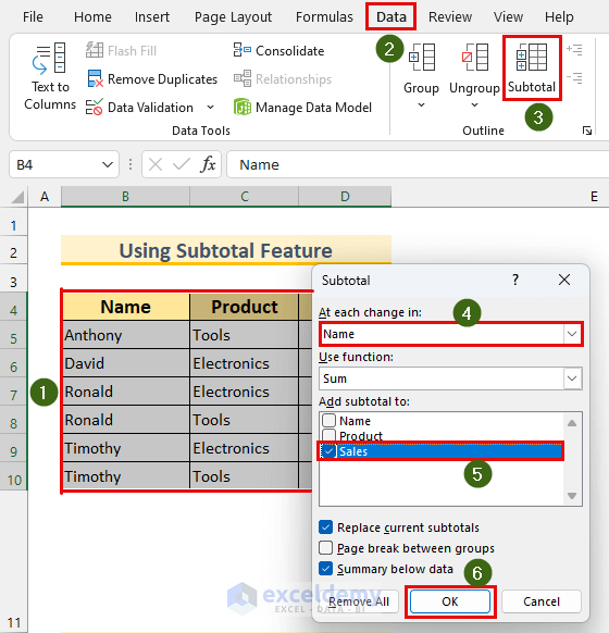
- Select the range B4:D10.
- From the Data tab, select Subtotal.
The Subtotal dialog box will appear.
- Select these:
- “At each change in:” as “Name”.
- “Add subtotal to:” as “Sales”.
- Tick “Summary below data”.
- Click OK.
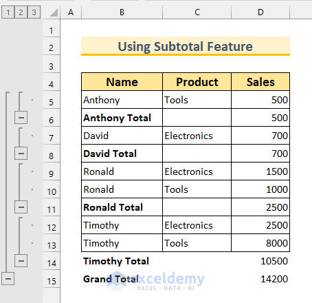
We’ve combined duplicate rows without losing data.
Method 6 – Combining UNIQUE and SUMIF Functions
Steps:
- Enter the following formula in cell B13:
=UNIQUE(B5:B10)This will extract the unique values from the cell range.
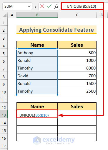
- Press ENTER. The cells will AutoFill.
- Select the range C13:C16 and enter this formula:
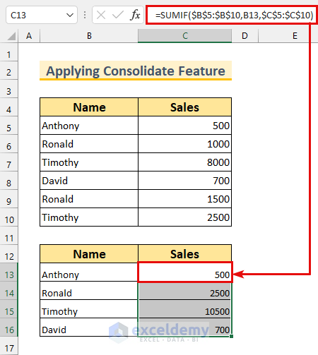
=SUMIF($B$5:$B$10,B13,$C$5:$C$10)We check in the range B5:B10 if there is a match with “Anthony”. If it is true, then we sum all the values, else the sum operation will not execute.
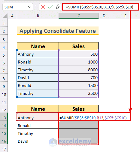
- Press CTRL + ENTER.
We’ve combined duplicate rows without any data loss.
Read More: Combine Duplicate Rows and Sum the Values in Excel
Things to Remember
- The UNIQUE function is only available in Microsoft 365 & Excel 2021.
- The TEXTJOIN function is only available from Excel 2019 version onwards.
- Use absolute cell references where it is necessary.
- For text values, we can use the first 2 methods. The last 4 methods are for numbers only.
<< Go Back to Merge Duplicates in Excel | Learn Excel
Get FREE Advanced Excel Exercises with Solutions!

