Let’s consider a scenario where a car dealer gives its cars code with this format: Car Model-Year. We have taken a dataset consisting of Car Model, Year, and Car Code as headers.
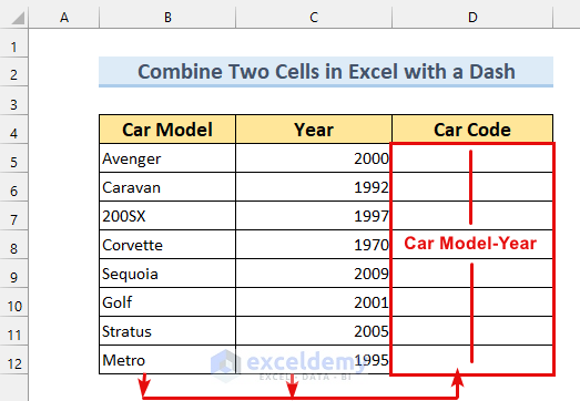
How to Combine Two Cells in Excel with a Dash: 5 Easy Ways
Method 1 – Using the Ampersand Operator to Combine Two Cells in Excel with a Dash
We can use the Ampersand symbol (&) for joining two cells.
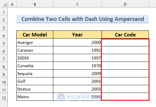
Steps:
- Select cell D5.
- Insert the following formula:
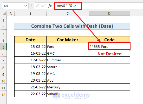
=B5&"-"&C5We are joining cells B5 and C5 with a dash (“-”) by using the Ampersand operator.
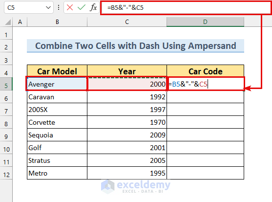
- Press Enter.
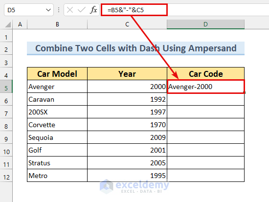
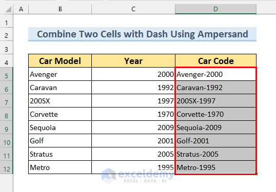
- The value of the two cells is combined with a dash.
- Move the cursor to the right-bottom corner of the cell to bring up the Fill Handle (+) icon.
- Drag down to AutoFill the cells with the formula.
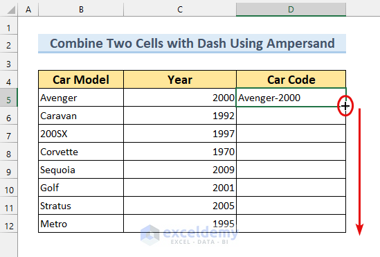
- The table should look like this.
Read More: How to Combine Cells into One with Line Break in Excel
Method 2 – Utilizing the CONCAT Function to Combine Two Cells in Excel with a Dash
If you have an older version of Excel, you can use the CONCATENATE function from method 4.
Steps:
- Use this formula in cell D5.
=CONCAT(B5,"-",C5)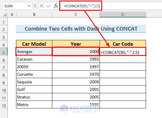
- Press Enter.
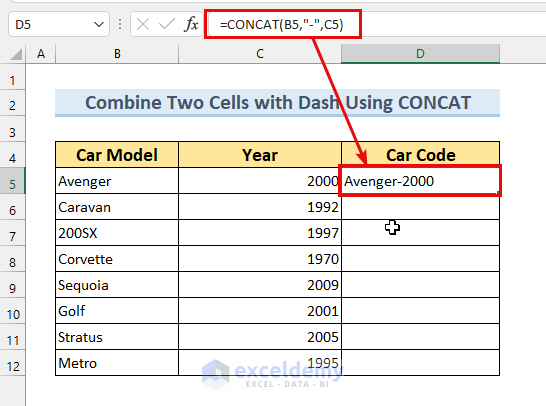
- Bring up the Fill Handle.
- Double Click on the icon (+).
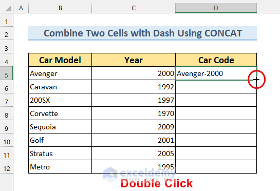
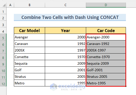
- The rest of the cells will be AutoFilled with the formula.
Read More: How to Concatenate Multiple Cells in Excel
Method 3 – Combine Two Cells in Excel with a Dash Using the TEXTJOIN Function
Steps:
- Select the cell range D5:D13.
- Enter the following formula:
=TEXTJOIN("-",TRUE,B5,C5)We are setting dash as our delimiter. The second value is set to TRUE, which means we’re ignoring the empty cells. You can set it to FALSE to include empty cells. The last two values are our two cells.
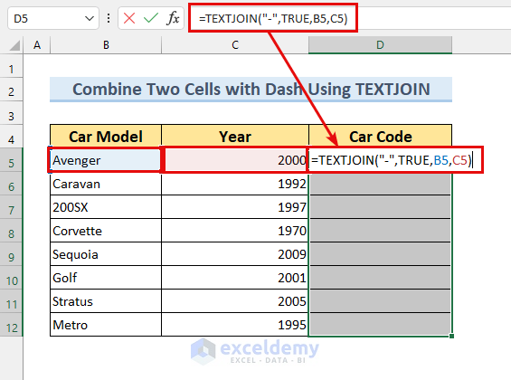
- Press Ctrl + Enter.
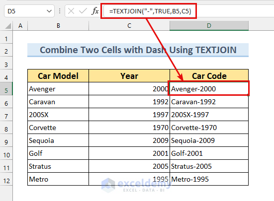
- This will Fill the formula into the selected cells.

- Here’s the result.
Read More: Concatenate Multiple Cells Based on Criteria in Excel
Method 4 – Applying the CONCATENATE Function to Combine Two Cells in Excel with a Dash
Steps:
- Use this formula in cell D5.
=CONCATENATE(B5,"-",C5)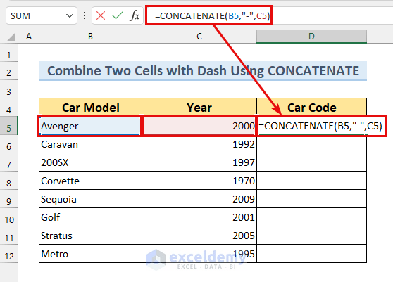
- Press Enter.
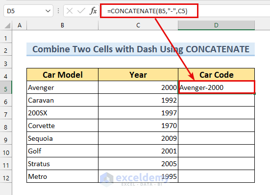
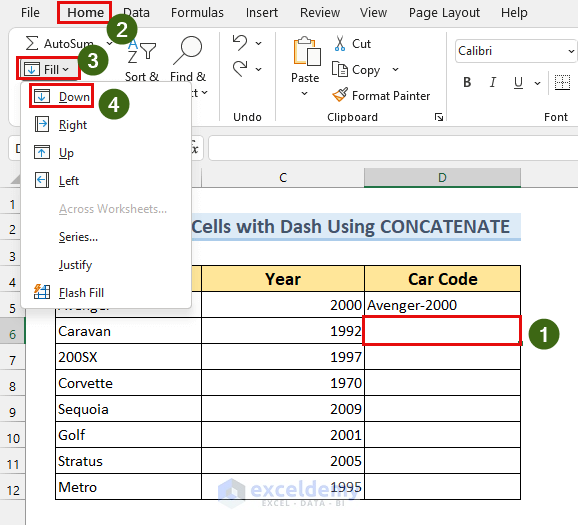
- You can use the Fill Handle to AutoFill the formula to the rest of the cells. You can also use the Fill Down command to do so too.
- Select cell D6.
- From the Home tab, select Fill then choose Down.
Alternatively, you can use Ctrl + D to fill down. You can do this for the rest of the cells.
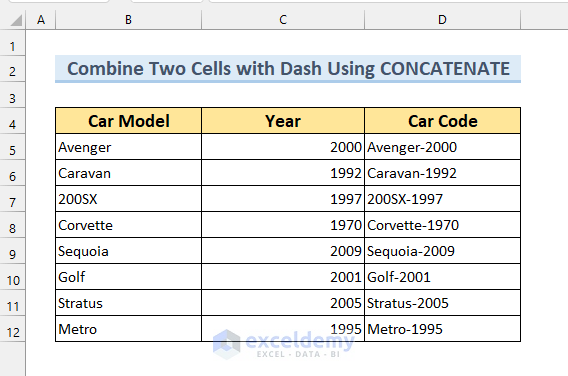
- Here’s the result.
Read More: Combine Multiple Cells into One Separated by Comma in Excel
Method 5 – Combine Text and Date with a Dash in Excel
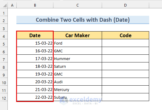
We have a new dataset with a list of the most commonly sold cars on a given date. We want to add those two columns to our Code column.
Before jumping into the steps, let’s see how the combination would look if we use our Ampersand method. We can see the date is in a weird format. To format the dates, we need to use the TEXT function.
Steps:
- Use this formula in cell D5.
=TEXT(B5,"dd-mm-yy")&"-"&C5The TEXT function will format cell B5 as date-month-year. Ampersand will join this formatted value with cell C5.
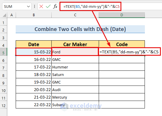
- Press Enter.
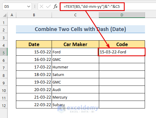
- AutoFill to the rest of the column however you want.
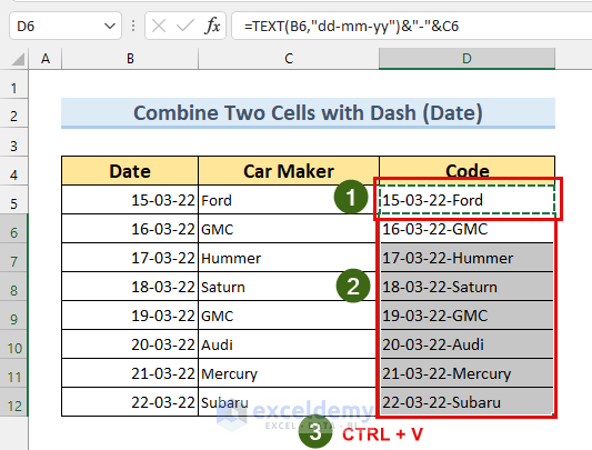
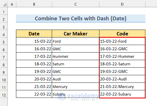
- Here’s the result.
Read More: Concatenate Multiple Cells but Ignore Blanks in Excel
Practice Section
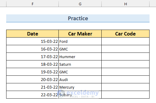
You can practice these methods using our provided practice tables in the Excel sheet.
Download the Practice Workbook
Related Articles
- How to Combine Cells with Same Value in Excel
- How to Merge Cells Using Excel Formula
- How to Merge Multiple Cells without Losing Data in Excel
- How to Merge Cells Vertically Without Losing Data in Excel
<< Go Back To Excel Concatenate Multiple Cells | Concatenate Excel | Learn Excel
Get FREE Advanced Excel Exercises with Solutions!

