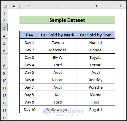
Consider the following dataset with 10 days of sales data from two different salesmen. Each of them sold one car per day which is given in columns B and C. We will compare these two columns to find out which models are sold by both of them on the same day or on different days.
Method 1 – Conditional Formatting to Compare Two Columns in Excel for a Match
Steps:
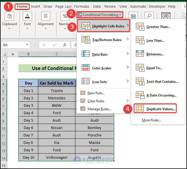
- Select the cells you want to compare.
- Go to Home and select Conditional Formatting.
- Choose Highlight Cells Rules and pick Duplicates Values.
- The Duplicate Values box will appear. Select Duplicate from the left side box and click on OK.
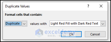
- You can change the format if you want but we’ll keep it as is.
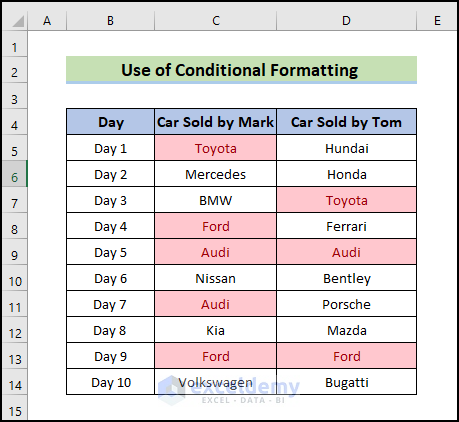
- The values that are common in both columns will be highlighted.
Method 2 – Finding a Match in Two Columns by Simple Formula
Steps:
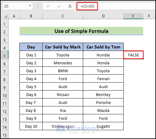
- To compare columns C and D, copy this formula in any empty cell in the row (E5),
=C5=D5
- Press Enter.
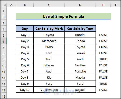
- If C5 and D5 have the same value, E5 will show TRUE. Otherwise, E5 will get FALSE.
- For our dataset, we have Toyota in cell C5 and Hundai in cell D5. They are different, so cell E5 is showing false.
- Drag cell E5 to the end of your dataset. It will apply the same formula in all other cells in column E.
Method 3 – Compare Two Columns with the VLOOKUP Function
Steps:
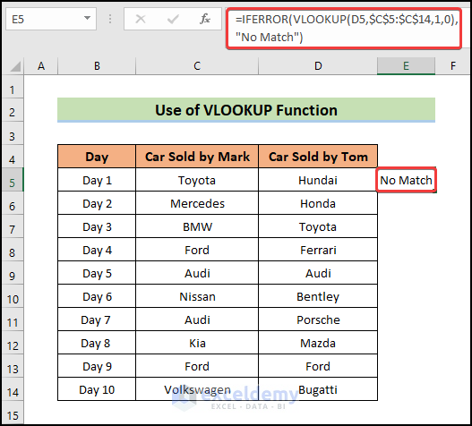
- Copy the following formula in cell E5:
=IFERROR(VLOOKUP(D5,$C$5:$C$14,1,0),"No Match")
- Press Enter.
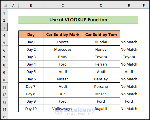
- If D5 has the same value as any of the values in Column C, E5 will show the value. If D5 has a unique value, E5 will show No match.
- For our dataset, Hundai is in cell D5, which is unique, so cell E5 is showing No match.
- Drag cell E5 to the end of your dataset.
- This will apply the same formula in all other cells in column E.
Method 4 – IF Function for Comparing Two Columns in Excel
Steps:
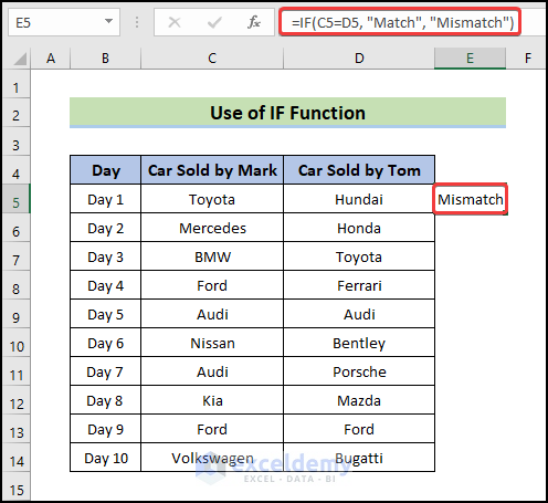
- To compare columns C and D, copy the following formula in the result cell for the row (E5):
=IF(C5=D5, "Match", "Mismatch")
- Press Enter.
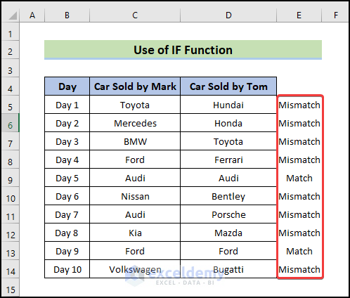
- Now, if the C5 and D5 cells have the same value, E5 will show Match. Otherwise, E5 will show Mismatch.
- For our dataset, we have Toyota in cell C5 and Hundai in cell D5. They are different, so cell E5 is showing Mismatch.
- Drag cell E5 to the end of your dataset.
- This will apply the same formula in all other cells in column E.
Method 5 – Compare Two Columns for a Match with the MATCH Function
Steps:
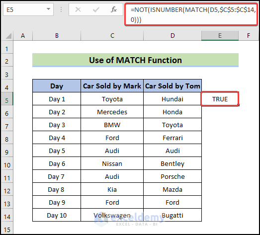
- Copy the following formula in cell E5:
=NOT(ISNUMBER(MATCH(D5,$C$5:$C$14,0)))
- Press Enter.
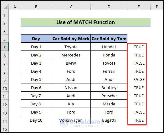
- If D5 has the same value as any of the values in Column C, E5 will show FALSE, and if D5 has a unique value, E5 will show TRUE.
- For our dataset, Hundai in cell D5 is unique, so cell E5 is showing TRUE.
- Drag cell E5 to the end of your dataset.
- This will apply the same formula in all other cells in column E.
Method 6 – Insert the INDEX Function to Compare Two Columns in Excel for a Match
Steps:
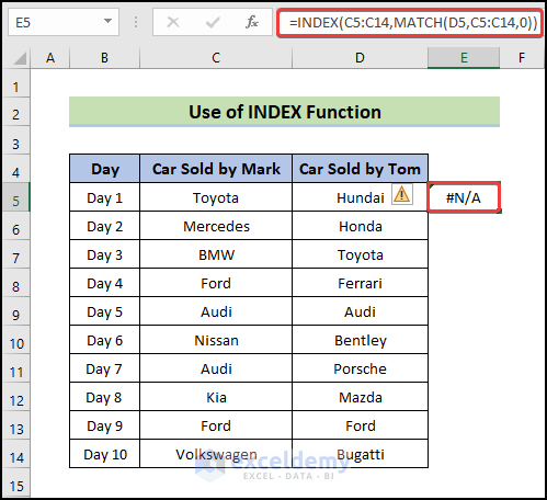
- Copy this formula in cell E5:
=INDEX(C5:C14,MATCH(D5,C5:C14,0))
- Press Enter.
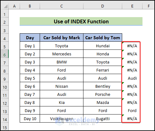
- If the C5 and D5 cells have the same value, E5 will show the value. Otherwise, you’ll get a #N/A error.
- For our dataset, we have Toyota in cell C5 and Hundai in cell D5. They are different, so cell E5 is showing #N/A.
- Drag the cell E5 to the end of your dataset. It will apply the same formula in all other cells in column E.
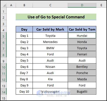
Method 7 – Compare Two Columns Through the Go to Special Command
Steps:
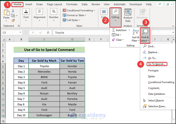
- Select the columns which you want to compare.
- Go to Home and select Editing.
- Choose Find & Select and pick Go to Special.
- The Go To Special box will appear.
- Select Row Difference and click OK.
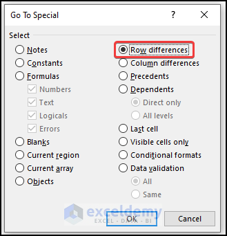
- All the unique values in column D will be highlighted.
Method 8 – Compare Two Columns with the EXACT Function
Steps:
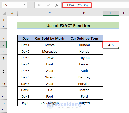
- To compare columns C and D, copy this formula in any empty cell in the row (E5),
=EXACT(C5,D5)
- Press Enter.
- For our dataset, we have Toyota in cell C5 and Hundai in cell D5. They are different, so cell E5 is showing false.
- Drag cell E5 to the end of your dataset.

Download Practice Workbook
You can download the following file to practice by yourself.


