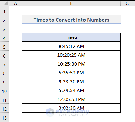
Suppose you have a list of time ranges. It contains the Times to Convert into Numbers.
Method 1 – Using Format Cells Option to Convert Time to Number in Excel
Let’s convert the times to the fraction of the day they represent.
Steps
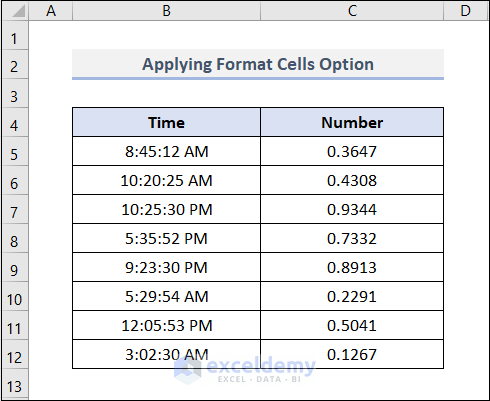
- Create a new column in the C4:C12 range.
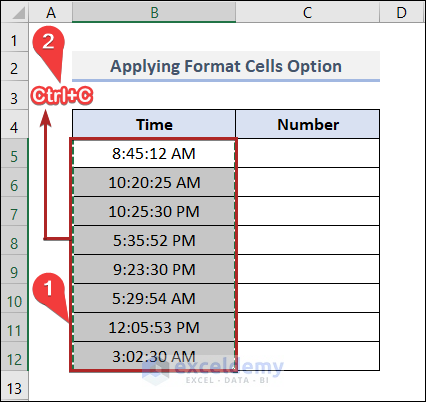
- Copy cells in the C5:C12 range by pressing CTRL+C.
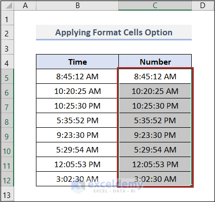
- Paste these into cell C5 with Ctrl + V.
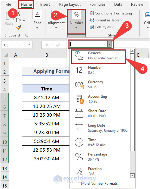
- Go to the Home tab.
- Select the Number group.
- Click on the drop-down arrow in the Number Format box.
- Choose the General format from the list.
- The times are showing as number values.
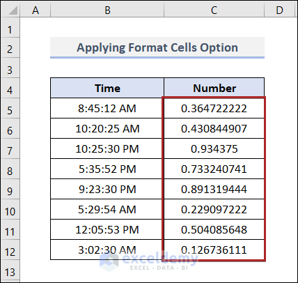
We can reduce the number of decimal digits to make it look nicer:
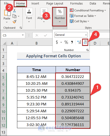
- Select cells in the C5:C12 range.
- Go to the Home tab.
- Select the Number group.
- Click several times on the Decrease Decimal icon until you get your desired digits after the decimal.
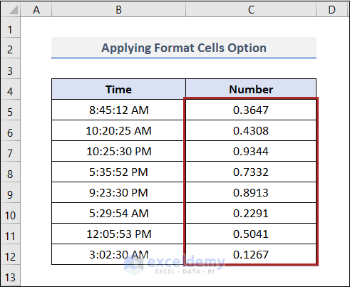
- We converted the times into numbers.
Read More: How to Convert Time to Decimal in Excel
Method 2 – Applying Excel TIMEVALUE Function to Convert Time to Number
We can also convert text values that represent time into numbers.
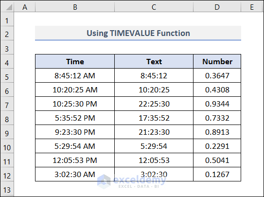
Steps
- Select cell C5.
- Write down the formula below and press Enter.
=TEXT(B5,"H:MM:ss")
In this formula, we used the TEXT function to convert the time in cell B5 into a text string.
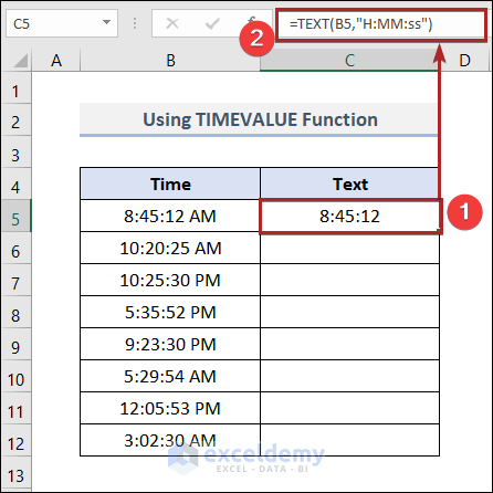
- Use the Fill Handle tool to copy the formula into the remaining cells.
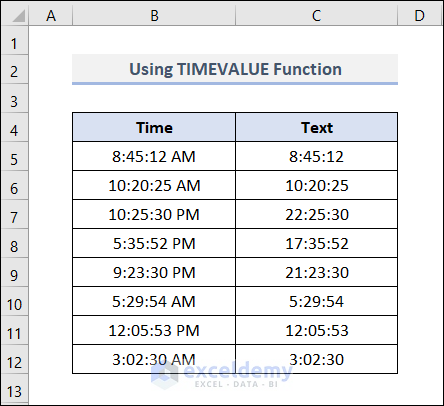
- Select cell D5 and type in the formula below.
- Press the Enter key.
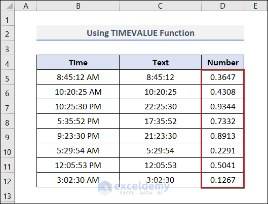
=TIMEVALUE(C5)
Here, C5 represents the text string 8:45:12 in cell C5.
Hence, we used the TIMEVALUE function here. This function takes a text string as input. Then, it returns the text string as a representation of time in decimal number format. The decimal value ranges from 0 to 0.99988426, which corresponds to the times between 0:00:00 (12:00:00 AM) and 23:59:59 (11:59:59 PM).
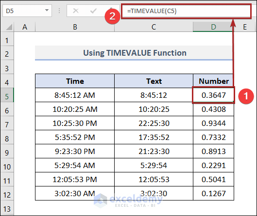
- The numbers look like the one below.
Read More: Convert Time to Text in Excel
Method 3 – Applying Simple Arithmetic Formula to Convert Time to Number
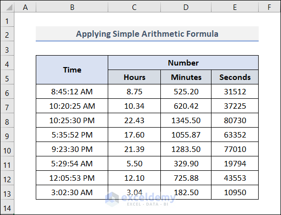
Let’s break down the time into how many hours, minutes, or seconds passed since midnight.
Steps
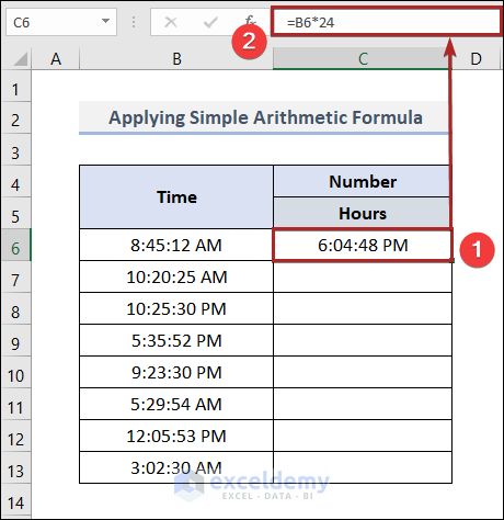
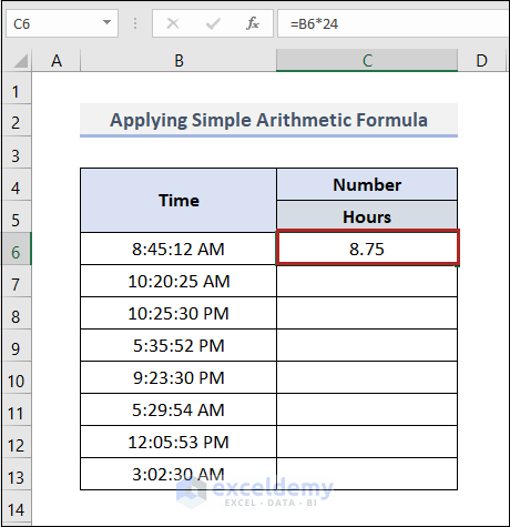
- Select cell C6.
- Write down the formula below and press Enter:
=B6*24
Here, B6 serves as the cell reference for the first Time in the list. In formula above, we multiplied B6 by 24 as this is the number of hours in a day.
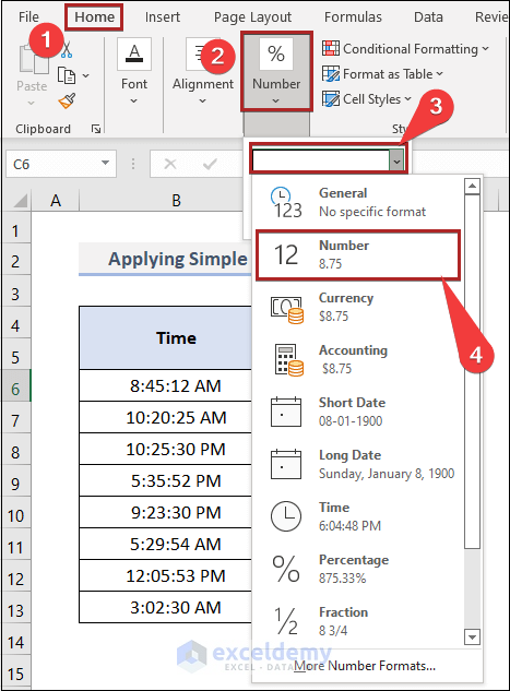
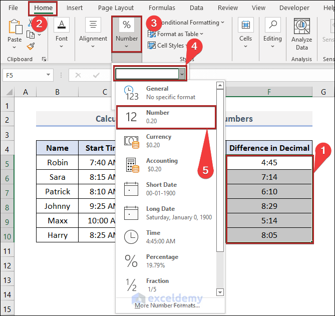
- Go to the Home tab.
- Select the Number group.
- Click on the down arrow in the Number Format box.
- Choose the Number format from the list.
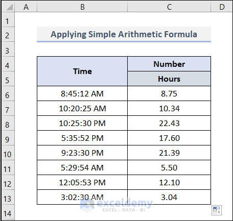
- The result is properly converted into the number of hours.
- Use the Fill Handle tool to get the full results.
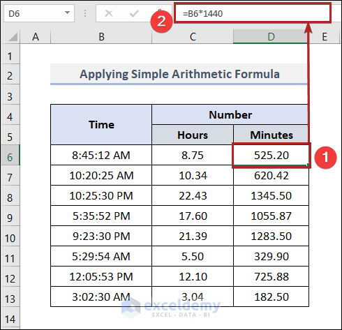
- Select cell D6 and paste down the formula below.
=B6*1440
Here, we multiplied the cell reference of B6 with 1,440 as it’s the number of minutes in a whole day.
- Press Enter.
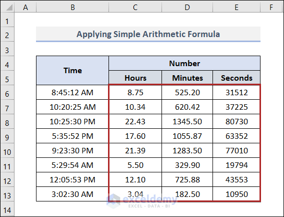
- Select cell F6.
- Copy the formula below and press Enter.
=B6*86400
We multiplied the value of cell B6 by 86,400 because it’s the number of seconds in a day.

- We converted the Time into the Number of Hours, Minutes, and Seconds.
Read More: How to Convert Time to Seconds in Excel
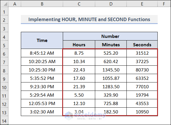
Method 4 – Combining Excel HOUR, MINUTE, and SECOND Functions to Convert Time to Number
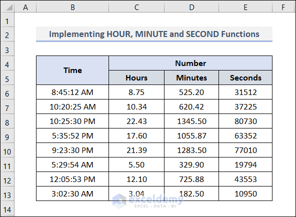
Steps
- Select cell C6 and put down the formula below.
=HOUR(B6)+MINUTE(B6)/60+SECOND(B6)/3600
Here, B6 serves as the cell reference for the first Time in the list.
⚙️ Formula Breakdown
- HOUR(B6) ⟶ The HOUR function returns the hour of a time value. Here, B6 is the serial_number argument. It is the time containing the hour we want to find.
- Output ⟶ 8
- MINUTE(B6)/60 ⟶ The MINUTE function returns the minutes of a time value. Then, we divided the output by 60 to get the result in hours.
- Output ⟶ 0.75
- SECOND(B6)/3600 ⟶ The Second function returns the seconds of a time value. The second is given as an integer in the range 0 to 59. We divided the output by 3600 to get it in hours.
- Output ⟶ 0
- Press the Enter key.
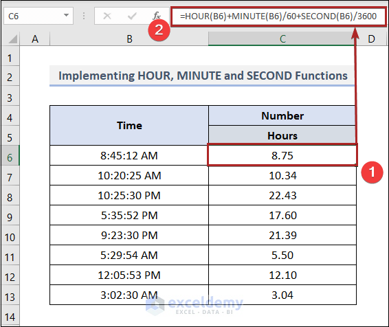
- Select cell D6 and put down the formula below:
=HOUR(B6)*60+MINUTE(B6)+SECOND(B6)/60
We’re calculating the number in minutes. So, we have to multiply the output of the HOUR function by 60. This converts the value from hours to minutes.
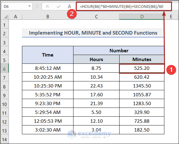
- Select cell E6 and paste the formula below:
=HOUR(B6)*3600+MINUTE(B6)*60+SECOND(B6)
- Press Enter.
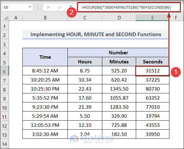
- We have converted the Time into Numbers of Hours, Minutes, and Seconds.
Method 5 – Use of CONVERT Function to Convert Time to Number in Excel
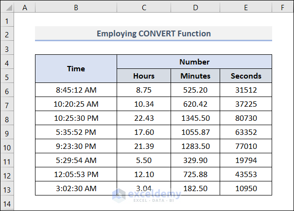
Steps
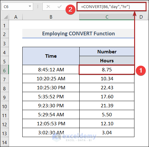
- Select cell C6 and write down the formula below:
=CONVERT(B6,"day","hr")
Here, B6 represents the time 8:45:12 AM.
In this function, the last two arguments are from_unit and to_unit. From_unit is the unit of the input. Whereas, to_unit is the unit for the result. In this case, the day is the from_unit and hr is the to_unit. This function converts the time of the day to just hours.
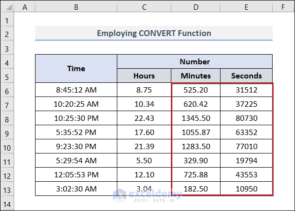
- Repeat the function in the other two columns, changing the to_unit argument to mn and sec, respectively.
Conversion of Time Difference to Numbers in Excel
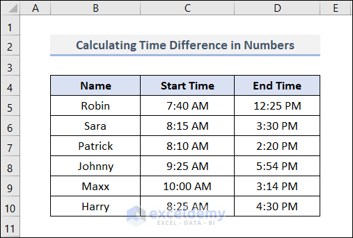
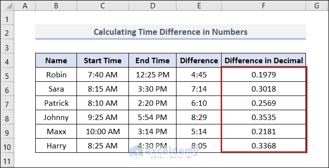
Consider a dataset containing the Start Time in Column C and End Time in Column D of a certain work.
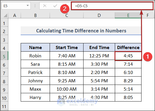
- Select cell E5 and paste down the formula below:
=D5-C5
Here, C5 and D5 serve as cell references for the first Start and End Time. These are 7:40 AM and 12:25 PM.
- Press the Enter key.
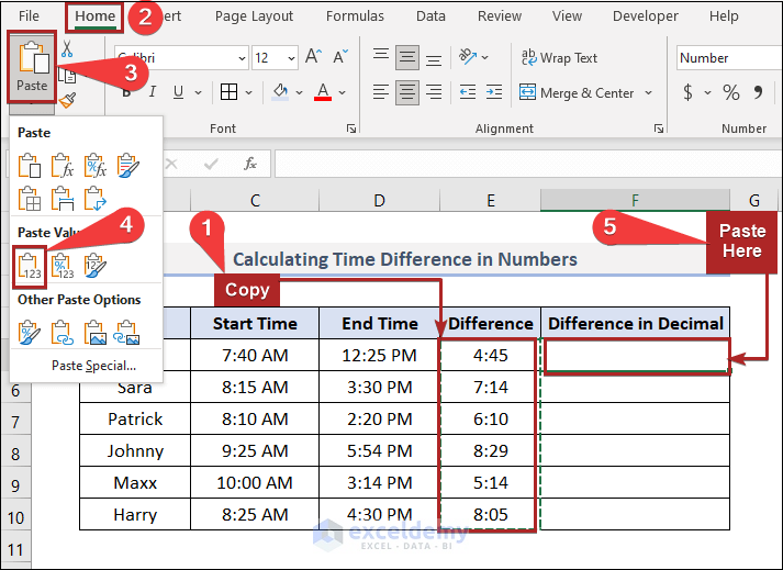
- Copy cells in the E5:E10 range.
- Go to the Home tab.
- Select Paste in the ribbon as per the image below.
- Select cell F5.
- Paste the copied data as Values (V).
- Change the cell format as in Method 3.
- The time difference is shown as numbers on the sheet.
Download Practice Workbook
You may download the following Excel workbook for better understanding and practice yourself.
Related Articles
- How to Convert Decimal Time to Hours and Minutes in Excel
- How to Convert Time to Hours in Excel
- Convert Military Time to Standard Time in Excel
- Convert Epoch Time to Date in Excel
<< Go Back to Time Conversion | Date-Time in Excel | Learn Excel
Get FREE Advanced Excel Exercises with Solutions!

