How to Copy and Paste in Excel When Filter Is On (5 Methods)

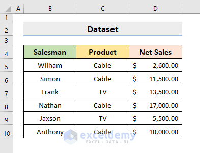
We’re going to use a sample dataset as an example. The following dataset represents the Salesman, Product, and Net Sales of a company. There are two products: Cable and TV. We’ll apply the Filter feature to the products.

How to Copy and Paste in Excel When the Filter Is on: 5 Methods

Method 1 – Keyboard Shortcuts to Copy and Paste When the Filter Is on in Excel

Steps:

• Select the range including the Headers.

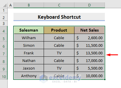
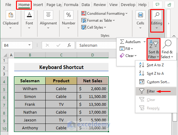
• Select Filter from the Sort & Filter drop-down list in the Editing group under the Home tab.

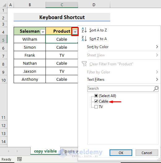
• Select the drop-down symbol beside the header Product.
• Check the Cable box only and press OK.

Case 1.1 – Copy Only the Visible Cells

STEPS:

• Select the range.

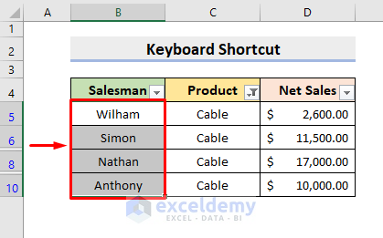
• Press Alt + ; to select only the visible cells.
• Press Ctrl + C to copy.
• Select cell F5 to paste the copied values.

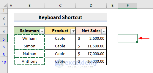
• Press Ctrl + V and Excel will paste the cells.

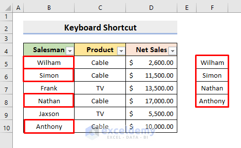
Case 1.2 – Paste a Value or Formula in the Visible Cells

Steps:

• Select cell F5 as this is the value we want to paste in the filtered column.

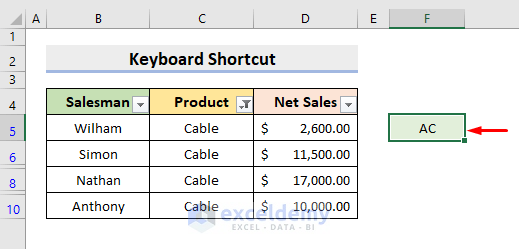
• Press Ctrl + C to copy.
• Select the cells in the filtered column where you want to paste the F5 cell value.

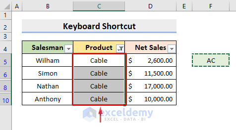
• Press F5 or Ctrl + G, and a Go To dialog box will pop out.
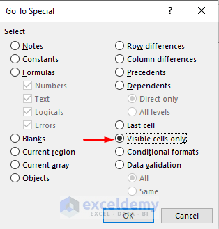
• Select Special.

• In the Go To Special dialog box, select Visible cells only and press OK.

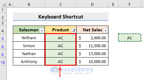
• Press Ctrl + V to paste the value.

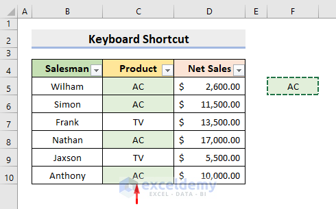
• If you remove the Filter feature, you’ll see the new value only in the visible cells of the previously filtered column.

Case 1.3 – Paste a Set of Values from Left to Right in a Filtered Table

Steps:

• Select the range.

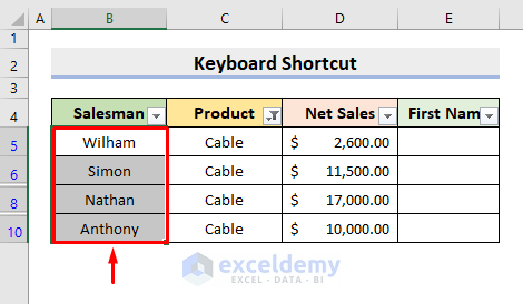
• Hold the Ctrl key and select the range of cells where you want to paste.

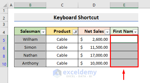
• Press Alt + ;.

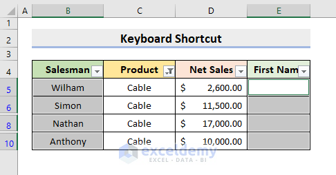
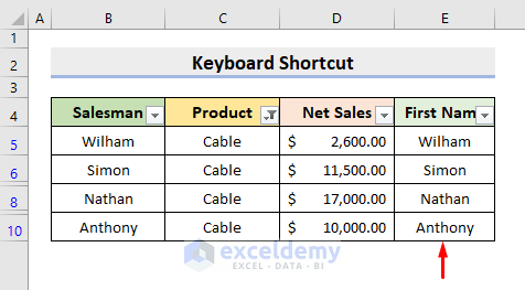
• Press Ctrl + R to paste the values in the required column.

Method 2 – Use the Fill Feature for Pasting a Set of Values from Right to Left in a Filtered Table

We applied a keyboard shortcut to paste a set of values from Left to Right in a filtered table. But, there is no such way to do that from Right to Left. We need a different method.

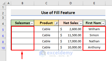
Steps:

• Select the range of cells.

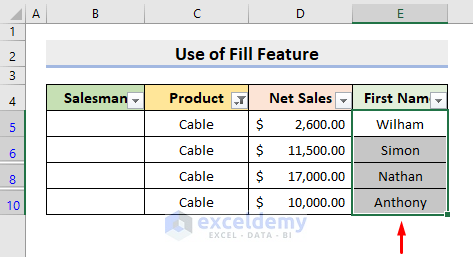
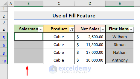
• Hold Ctrl and select the column in the left where you want to paste.
• Press Alt + ; to select only the visible cells.

• Select Left from the Fill drop-down list in the Editing group under the Home tab.

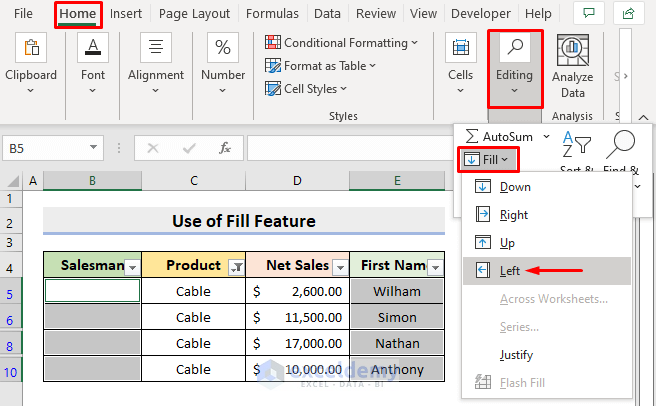
• This will paste the values in the selected column on the left side.

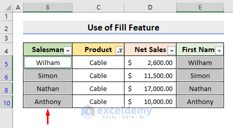
Method 3 – Excel Find & Select Feature to Copy Only the Visible Cells in a Filtered Column

Steps:

• Select the range you want to copy.

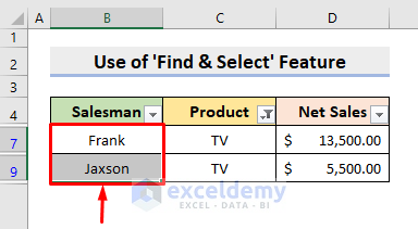
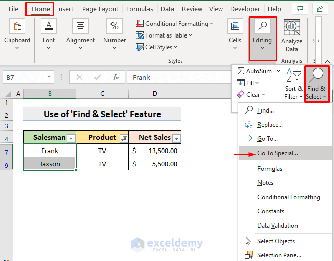
• Under the Home tab, select Go To Special from the Find & Select drop-down list in the Editing tab.

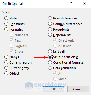
• Select Visible cells only.
• Press OK.

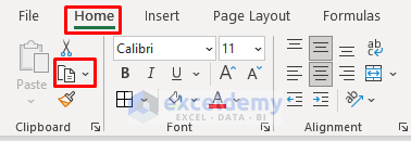
• Select Copy in the Clipboard section.

• Select any cell you where you want to paste.
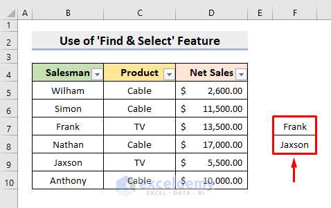
• Press Ctrl + V.

Method 4 – Apply a Formula to Paste a Set of Values to the Visible Cells

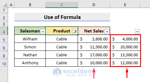
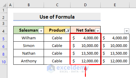
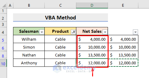
We want to copy the values in column E and paste them into column D only for the product Cable.

Steps:

• Apply a filter to select only rows with Cable for Product.
• Select cell D5 and insert the formula:

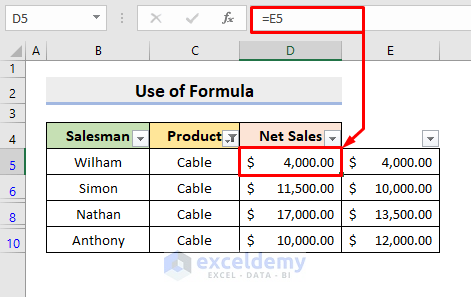
• Press Enter and use the AutoFill tool to fill the series.
• It’ll simply paste the values.

Read More: Copy and Paste Formulas Without Changing Cell References

Method 5 – Paste a Set of Values with Excel VBA When the Filter Is On

STEPS:

• Under the Developer tab, select Visual Basic.

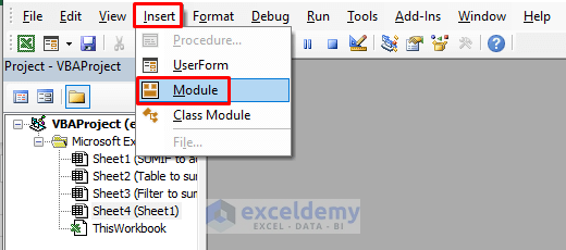
• Under the Insert tab, select Module.

• A new window will pop out.
• Paste in the code given below:

Sub Paste()
Dim rg As Range
Dim visible_source As Range
Dim destination As Range
Dim source As Range
Dim r As Range
Set rg = Application.Selection
rg.SpecialCells(xlCellTypeVisible).Select
Set visible_source = Application.Selection
Set destination = Application.InputBox("Choose Destination:", Type:=8)
For Each source In visible_source
source.Copy
For Each r In destination
If r.EntireRow.RowHeight <> 0 Then
r.PasteSpecial
Set destination = r.Offset(1).Resize(destination.Rows.Count)
Exit For
End If
Next r
Next source
End Sub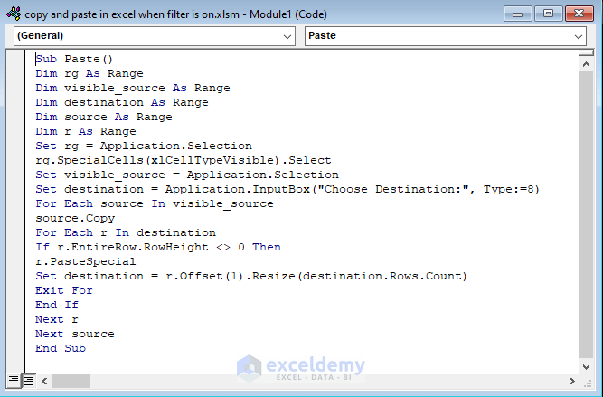

• Close the Visual Basic window.
• Select the range to copy.

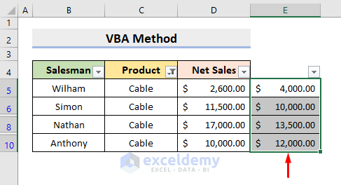
• Select Macros under the Developer tab.

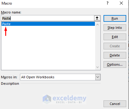
• A Macro dialog box will open.
• Select Paste in the Macro name and press Run.

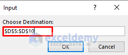
• Another dialog box will pop out asking to choose the destination.
• In the Choose Destination box, type $D$5:$D$10 or select the range of cells in the table where you want to paste the values, then press OK.

• The required output will appear in column D.

Read More: Copy and Paste Without Changing the Format in Excel

Download the Practice Workbook

Related Articles

<< Go Back to Copy Paste in Excel | Learn Excel