Copy Pivot Table Data to Another Worksheet Without Pivot in Excel

In Excel, Pivot Table is one of the most powerful tools, especially for large datasets. It helps to summarize, organize and filter values from the huge data string. But sometimes after creating a pivot table, we need to copy it to another worksheet but not as a pivot. The process only keeps the values and formatting of the original one. There are several ways to copy pivot table data without a pivot in Excel. In this article, we will describe 4 useful methods to do it.

What Is Pivot Table in Excel?

You may have thousands of data in your worksheet which makes it really confusing to understand. This is where we need a Pivot Table. A pivot table is a tool in Microsoft Excel that helps to explore this huge dataset in a summarized, precise pattern. It helps to filter according to groups, labels or categories for better understanding. Even you can expand or collapse and rotate rows and columns to get data in various dimensions. It also gives you cumulative totals for certain values.

Copy Pivot Table Data to Another Worksheet Without Pivot in Excel: 4 Useful Methods

To copy a pivot table, we need to create one first. For this, follow the quick steps below.

• In the beginning, we created a dataset where 4 cities’ have various amounts of Sales and Profit on different Dates.

• Then, select this whole dataset and go to the Insert tab.
• Here, select From Table/Range under the PivotTable section.

• Following, select the Location where you want to get the pivot table and hit OK.

• Afterward, place your required fields in their respective sections according to your preference like this.

• That’s it, we have our desired pivot table beside our original dataset.

Now, let us follow the methods below to copy this pivot table to another worksheet without pivot features.

1. Use Paste Special Feature to Copy Pivot Table Data Without Pivot

In this first method, we will apply the Paste Special feature of Excel to copy pivot table data. To do the task, follow the steps below.

• First, select your whole pivot table and press Ctrl + C to copy it.

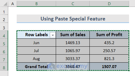
• Then, go to the new worksheet and select a cell where you want to copy it.
• Afterward, right-click on it and click on Paste Special.

• Next, you will see the Paste Special dialogue box.
• Here, select Values in the Paste category and press OK.

• Following, you will see that there are only the values fetched from the pivot table.

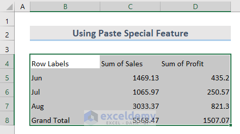
• Now, select the cell range B4:D8 and right-click again.
• Then, select Formats in the Paste section.

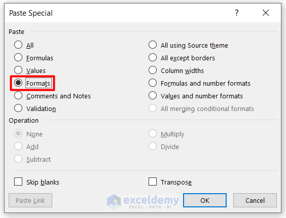
• Lastly, press OK and you will get the pivot table without pivot in another worksheet.

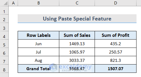
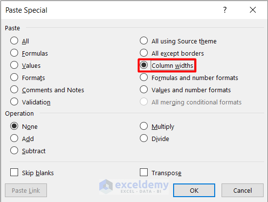
• Moreover, if you need to match the column width with the original one, simply select Column widths in the Paste Special window after completing the above steps.

2. Apply Clipboard Tool to Copy Data Without Pivot in Excel

Another quick way is to use the Clipboard tool in Excel for copying pivot table data. Among all, this is the fastest method for the process.

• In the beginning, select the whole pivot table that we created earlier.

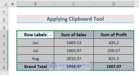
• Then, go to the new worksheet and select the cell where you want to get the input.
• Following, click on the Clipboard icon under the Home tab.

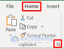
• After this, you will see that the Clipboard panel appears on the left.
• Here, select the Item for pasting from the list.

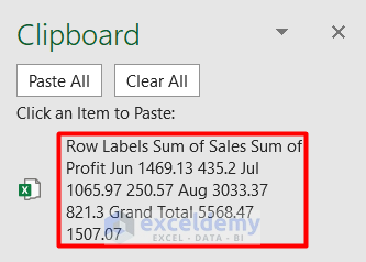
• Finally, you will get the pivot table data without pivot like this.

3. Excel VBA to Copy Pivot Table Data Without Pivot

Using Excel VBA Macro code is another useful technique for copying pivot table data to another worksheet. To conduct the task, go through the steps below.

• First, select any cell in the pivot table.
• Then, go to the Developer tab and select Visual Basic under the Code group.

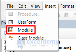
• Next, in the Visual Basic window, select Module from the Insert tab.

• After this, insert this code in the blank page.

Sub PivotTableCopy()
Dim wst As Worksheet
Dim pivot As PivotTable
Dim rgPT As Range
Dim rgPTa As Range
Dim rgCopy As Range
Dim rgCopy2 As Range
Dim lRwTop As Long
Dim lRwsPT As Long
Dim lRwPage As Long
Dim msgSpc As String

On Error Resume Next
Set pivot = ActiveCell.PivotTable
Set rgPTa = pivot.PageRange
On Error GoTo errorHandler

If pivot Is Nothing Then
    MsgBox "Unable to copy"
    GoTo extHandler
End If

If pivot.PageFieldOrder = xlOverThenDown Then
  If pivot.PageFields.Count > 1 Then
    msgSpc = "Horizontal filters with spaces or blank cells." _
      & vbCrLf _
      & "Unable to copy Filters formatting."
  End If
End If

Set rgPT = pivot.TableRange1
lRwTop = rgPT.Rows(1).Row
lRwsPT = rgPT.Rows.Count
Set wst = Worksheets.Add
Set rgCopy = rgPT.Resize(lRwsPT - 2)
Set rgCopy2 = rgPT.Rows(lRwsPT)

rgCopy.Copy Destination:=wst.Cells(lRwTop, 2)
rgCopy2.Copy _
  Destination:=wst.Cells(lRwTop + lRwsPT - 2, 2)

If Not rgPTa Is Nothing Then
    lRwPage = rgPTa.Rows(1).Row
    rgPTa.Copy Destination:=wst.Cells(lRwPage, 1)
End If
    
wst.Columns.AutoFit
If msgSpc <> "" Then
  MsgBox msgSpc
End If

extHandler:
    Exit Sub
errorHandler:
    MsgBox "Unable to copy"
    Resume extHandler
End Sub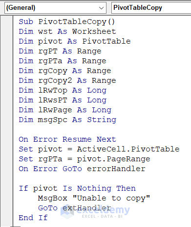

• Following, click on the Run Sub button or press F5 on your keyboard.

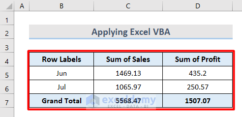
• Finally, you will successfully copy the pivot table data to another worksheet.

4. Copy Pivot Data with Report Filters to Another Worksheet

In this last method, we will copy pivot table data that has report filters with it. Report filters are the signified categories that we get in the PivotTable Fields. Now, follow the process below to copy data to another worksheet without pivot.

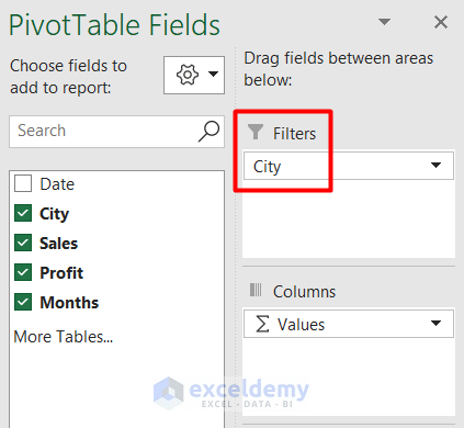
• In the beginning, drag the City title to the Filter category to specify it as a Report Filter.

• Afterward, you will get the Report Filter along with the pivot table like this.

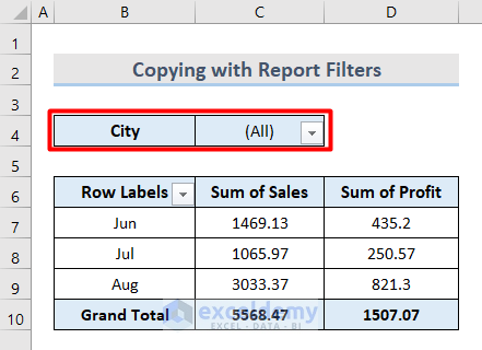
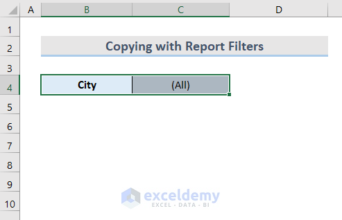
• Now, select the cell range B4:C4 that has the Report Filter and press Ctrl + C to copy it.
• Then, go to the new worksheet and select a cell.
• Following, press Ctrl + V to place the copy.

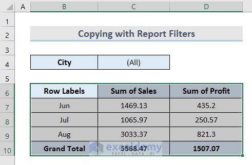
• Similarly, copy the pivot table by pressing Ctrl + C again.
• Finally, press Ctrl + V to paste it into the new worksheet.

Things to Remember

• In the case of the Report Filter, do not select any blank cells while copying.
• If multiple Report Filters are arranged horizontally, you cannot copy the pivot table data during running the VBA code. Otherwise, you will see an error message regarding this issue.
• Following any of the methods above benefits you with small file size, but may lose some sensitive data of the original pivot table.

Download Practice Workbook

Get this sample file to try the methods by yourself.

Conclusion

Concluding the article, hoping that it was helpful for you. Go through the tutorial carefully and copy pivot table data to another worksheet without the pivot with 4 useful methods. Let us know your insightful suggestions in the comment box.

Related Article

• How to Copy and Paste Pivot Table Values with Formatting in Excel

<<Go Back to How to Copy Pivot Table| Pivot Table in Excel | Learn Excel