How to Copy Unique Values to Another Worksheet in Excel – 5 Methods

The dataset showcases a list of colors with duplicates in Sheet1. To copy the unique colors to another worksheet in the same workbook.

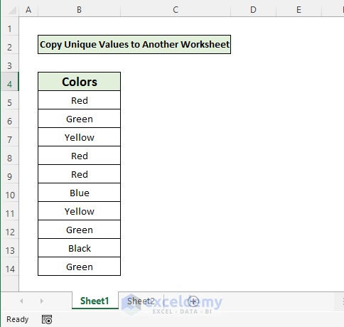
Method 1 – Copy the Unique Values to Another Worksheet Using the Advanced Filter Option in Excel

To copy the list of unique colors from Sheet1 to Sheet2:

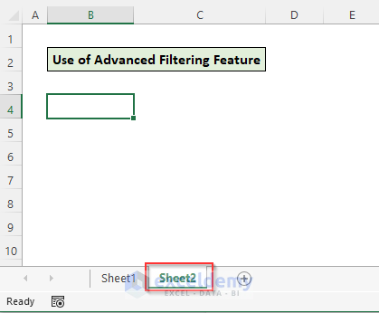
Steps:

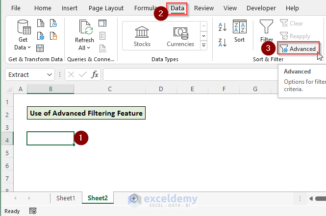
• Select B4 in Sheet2.
• Go to the Data tab.
• In Sort & Filter, click Advanced.

• In the Advanced Filter window, check “Copy to another location” and “Unique records only”.

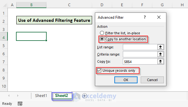
• Click the arrow sign to select the List range.

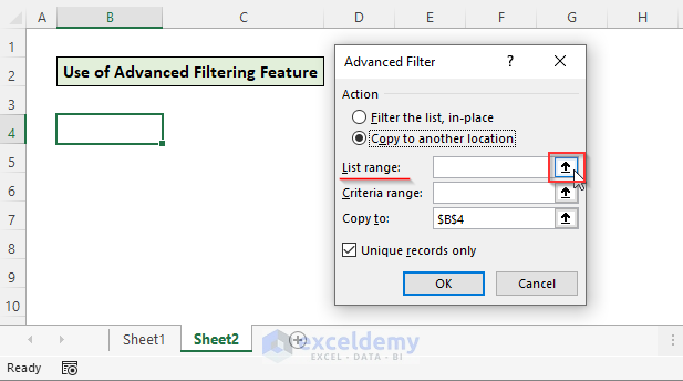
• Click Sheet1.

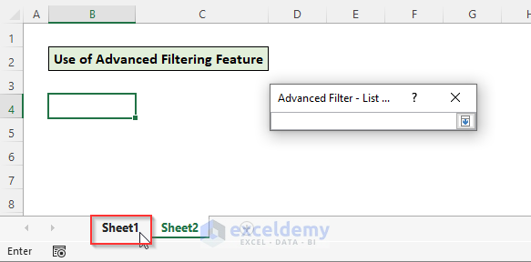
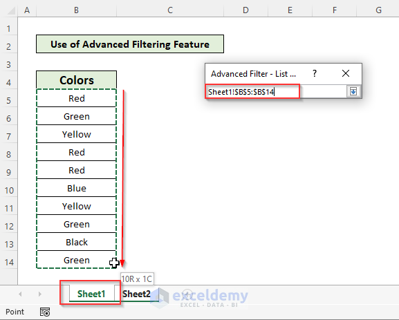
• Select B5:B14 and and drag the cell range into the input box.
• Press Enter.

• In the Advanced Filter window, click OK.

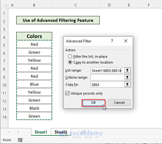
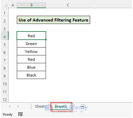
The unique list of colors is copied to Sheet2.

Method 2 – Using the UNIQUE Function to Copy Unique Values to Another Worksheet in Excel

To copy the list of unique colors from Sheet1 to Sheet3:

Steps:

• Select B5 in Sheet3 and enter the UNIQUE function.
• To enter the array argument of the function, click Sheet1.

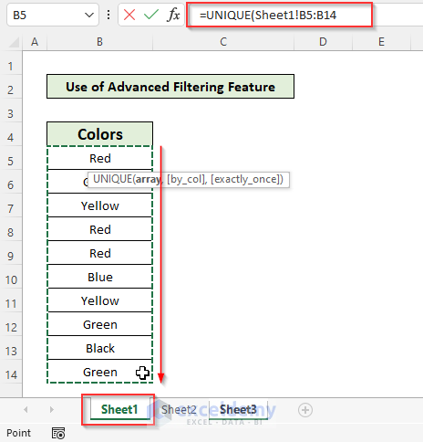
• Select B5:B14 in Sheet1.

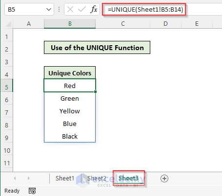
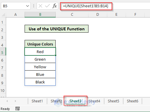
• Close the parenthesis and press Enter.

Method 3 – Applying the INDEX MATCH Array Formula to Copy Unique Values to Another Worksheet in Excel

To copy unique values from Sheet1 to Sheet4, this is the general formula:
=INDEX(mainList, MATCH(0, COUNTIF(uniqueList,mainList), 0))

• Enter the following formula in B5, Sheet4
• Press Ctrl + Shift + Enter.

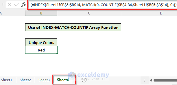
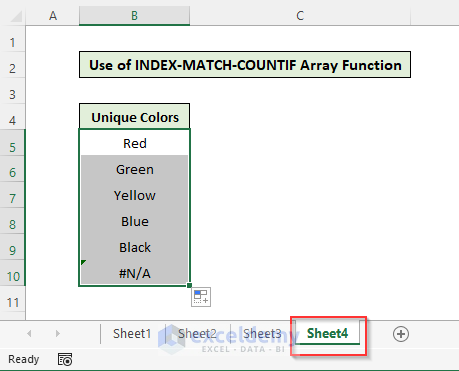
• Drag down the Fill Handle until it returns an error.

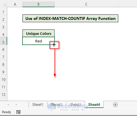
This is the output.

Formula Breakdown

The INDEX function needs two arguments – array and row_num. It returns a value to add to the unique list.
array – is the list of colors in Sheet1 (Sheet1!$B$5:$B$14).

row_num– The MATCH function finds the colors that are not in the unique color list. It returns the first match if there are duplicates.

The COUNTIF function counts how many times a color in the unique list in Sheet4 appears in the main color list in Sheet1. Here, $B$4:B4 is the expanding reference to look for colors in the unique list in Sheet4 and in the main list Sheet1!$B$5:$B$14 in Sheet1.

Method 5 – Using the LOOKUP Function to Copy Unique Values in Excel

To copy unique values to another worksheet, this is the general formula:

=LOOKUP(2,1/(COUNTIF(uniqueList,mainList)=0), mainList)

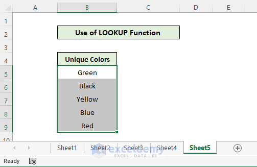
The color list in Sheet1 is the mainList and an expanding reference $B$4:B4 is used in Sheet5.

The formula becomes:

• Enter the formula in B5, Sheet5.

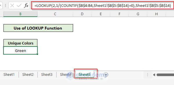
• Drag down the Fill Handle to see the result in the rest of the cells.

Method 5 – Copy Unique Values to Another Worksheet Using a VBA Code in Excel

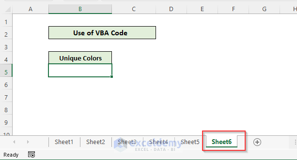
Steps:

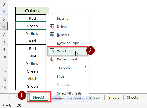
• Go to Sheet1 and right-click the name tab.
• Choose View Code.

• Enter the following code in the visual code editor and press F5 to Run the code.

Sub UniqueValue()
Dim WSheet1 As Worksheet
Dim Rng As Range
Dim WSheet2 As Worksheet
Set WSheet1 = Worksheets("Sheet1")
Set Rng = WSheet1.Range("B5:B" & WSheet1.Range("B65536").End(xlUp).Row)
Set WSheet2 = Worksheets("Sheet6")
Rng.Cells(1, 1).Copy WSheet2.Cells(5, 2)
Rng.AdvancedFilter Action:=xlFilterCopy, CopyToRange:=WSheet2.Range("B5"), Unique:=True
End Sub

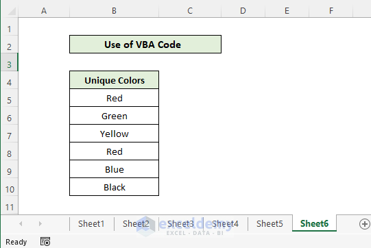
• Go to Sheet6.

This is the output.

Code Breakdown

In line 1, the range is set as B5 to the end of column B in Sheet1:  the color list is in B5:B14 in Sheet1.
In line 2, the worksheet to copy the unique values is set as Sheet6.
Line 3 defines the first unique value to be copied: cell(5,2) B5 in Sheet6.
In line 4, the filtering criteria are set and enabled Unique to True.

Notes

• To avoid the #N/A error in method 2 and method 3, use the IFERROR function in the formula. The formula becomes:

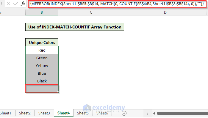
• Press Ctrl + Shift + Enter to apply an array formula.

Download Practice Workbook

Download the practice workbook to exercise.

<< Go Back to Learn Excel