We have a dataset here with information on fruit names and their amounts. We want to find the number of cells that have the name Apple in them.

Method 1 – Count Cells with Specific Text Using the COUNTIF Function
Case 1.1 – Partial Match
- Insert this formula in cell C17.
=COUNTIF(B5:B15,"*Apple*")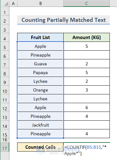
- Press Enter.
- You will see the number of cells that contain the text Apple. It also extracted text from Pineapple.
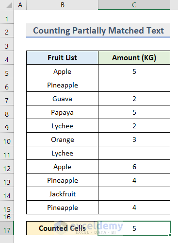
We used the COUNTIF function to count cell range B5:B15 to meet the single condition of finding the text Apple. We inserted the Wildcard (*) for partial matching.
=COUNTIF(B5:B15,"*"&B5&"*")
Case 1.2 – Exact Match
- Insert this function in cell C17.
=COUNTIF(B5:B15,"Apple")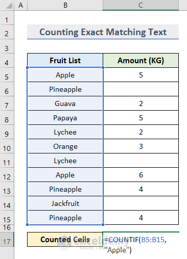
- Hit Enter.
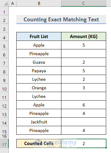
=COUNTIF(B5:B15,B5)
Read More: How to Apply COUNTIF When Cell Contains Specific Text
Method 2 – Apply Data Validation to Count Specific Text Cells in Excel
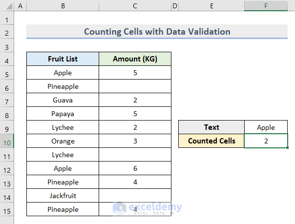
- Select cell F9 because we will insert the Data Validation command here.
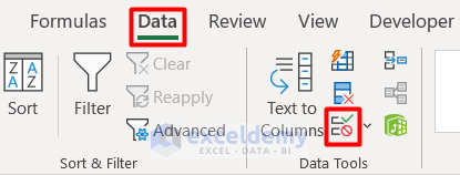
- Go to the Data tab and select Data Validation under the Data Tools group.
- Select List for Allow group and cell range B5:B15 in the Source box.
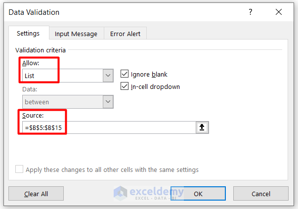
- Press OK.
- You will see an arrow beside cell F9.
- Select the specific text from the drop-down list.
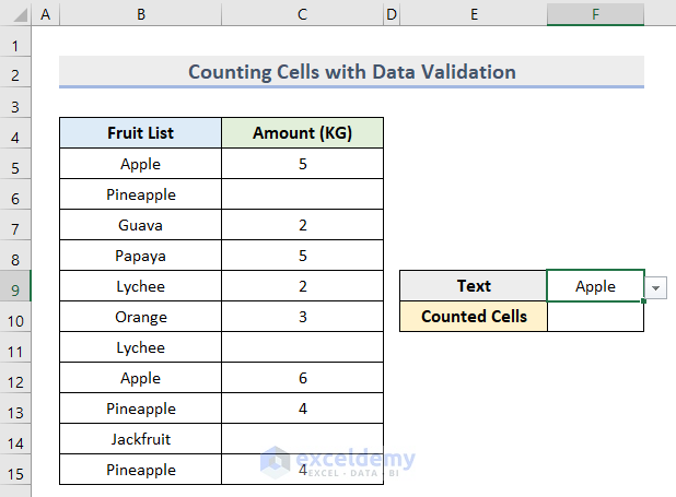
- Insert this formula in cell F10.
=COUNTIF(B5:B15,F9)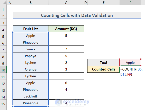
- Hit Enter to see the final output.
Method 3 – Insert the SUMPRODUCT Function for Counting Cells with Specific Text
- Insert this formula in cell C17.
=SUMPRODUCT(--(ISNUMBER(FIND("Apple",B5:B15))))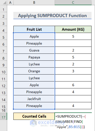
- Hit Enter.
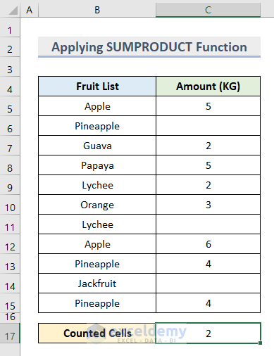
We applied the SUMPRODUCT function to return the products’ sum from cell range B5:B15. We used the ISNUMBER function to check if the reference value “Apple” is a number or not. We applied the FIND function to search for the specific text from the data string.
=SUMPRODUCT(--(ISNUMBER(FIND(B5,B5:B15))))
Method 4 – Count Cells with Specific Text Using Excel VBA
- Click on Visual Basic under the Developer tab.

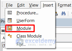
- Select Module from the Insert section.
- Insert this code on the blank page.
Sub COUNT_TEXT()
Dim iVal As Integer
iVal = Application.WorksheetFunction.CountIf(Range("B5:B15"), "Apple")
MsgBox iVal
End Sub
<img class="aligncenter wp-image-224403 size-full" src="https://www.exceldemy.com/wp-content/uploads/2018/06/Excel-Count-Cells-with-Specific-Text-15-1.png" alt="Excel VBA to Count Cells with Specific Text" width="732" height="210" />
You can edit the range and specific text to perform in your worksheet.
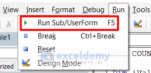
- Click on Run Sub or press F5 on your keyboard.
- Click on Run in the Macros window.

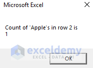
- You will see the number of cells in a message box like this:

Sub COUNT_ROWS()
For j = 1 To 12  'Adjust Rows
  count = 0
  For i = 1 To 2 Step 12 'Adjust Columns
    If Cells(j, i) = "Apple" Then count = count + 1
  Next i
  MsgBox "Count of 'Apple's in row " & j & " is " & vbLf & count
Next j
End Sub
A text box appears with the number of repetitions in row 1. After pressing OK, it will tell you the number of appearances of the text value in row 2. The process continues for all rows.
Read More: Excel VBA to Count Cells Containing Specific Text
Method 5 – Specific Text Cell Counting with the Filter Option in Excel
- Select cell range B4:C15.
- Go to the Data tab and select Filter from the Sort & Filter group.

- Filter your dataset according to your preference.
- Insert this formula in cell 18.
=SUMPRODUCT(SUBTOTAL(103, INDIRECT("C"&ROW(C5:C15))), --(B5:B15=C17))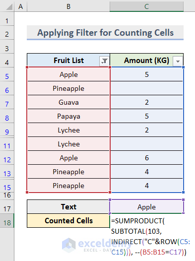
- Press Enter.
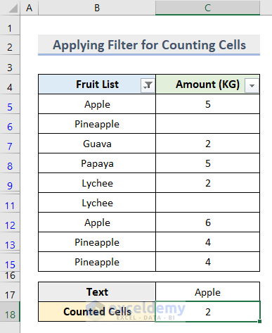 We applied the SUMPRODUCT function to get the sum of the dataset. We applied the SUBTOTAL function for getting total cumulative data. We provided the INDIRECT function to lock cell C17. We used the ROW function to select the rows from the dataset.
Read More: How to Count Filtered Cells with Text in Excel
How to Count Cells with All Types of Text in Excel
- Insert this formula in cell C17.
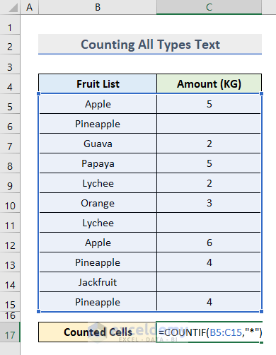
- Hit Enter.
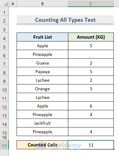
=SUMPRODUCT(--(ISTEXT(B5:C15)))
Read More: How to Count Cells in Excel with Different Text
How to Count Cells with Multiple Substrings in Excel
We want to calculate the number of cells filling more than one text criterion. We have a list where different items are listed along with their color and size. We want to count the item T-Shirt with the color blue.
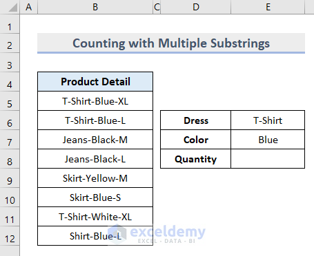
- Insert this formula in cell E8.
=COUNTIFS(B5:B12,"*T-Shirt*", B5:B12,"*Blue*")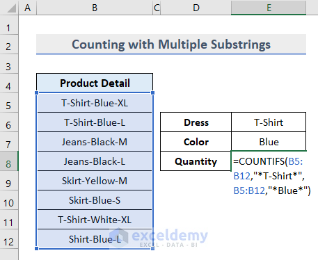
- Hit Enter and you will see the final output.
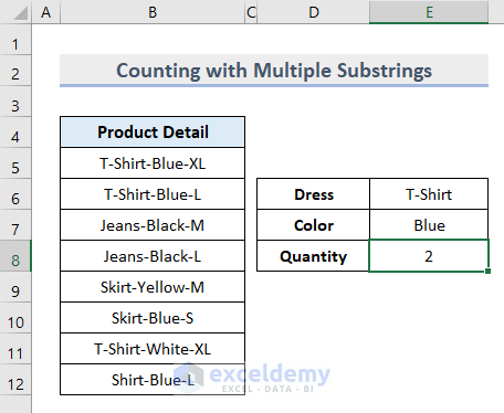
=COUNTIFS(B5:B12,"*"&E6&"*", B5:B12,"*"&E7&"*")
Download the Practice Workbook
Get FREE Advanced Excel Exercises with Solutions!


very intresting account always thought there was a way to handle the need. If I can here’s a question I have tried to have the sheet highlight data in cells but every time I it doesn’t work out. Can you possibly cover that if you haven’t yet. Thanks in advance
Hi DAVID BAKER! Hope you are well!
This article will help you to highlight specific data in cells.
https://www.exceldemy.com/highlight-specific-text-in-excel-cell-vba/
Best Regards.
I was able to add conditional formatting by using the same formula. Where A2 used a formula to determine which cells to format, and the formula → =COUNTIF(A3:A3,”*Apple*”)=1
Then copied this to the column.
Thanks for your input, Greg.
Best regards