Method-1 – Use of COUNTIF Function to Count Rows with Any Text
To count the number of texts in the Size column you have to use the COUNTIF function here. We added a column named Count for counting the number of texts.
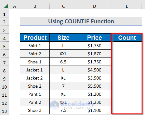
Steps:
➤ Sselect the output cell in the Count column.
➤ Type the following function here:
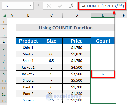
=COUNTIF(C5:C13,"*")C5:C13 is the range, and * is the wildcard that matches any number of text characters.
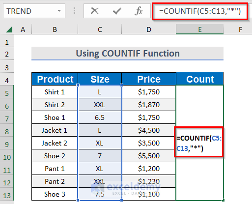
➤Press ENTER.
➤ The value of texts in the Size column.
Method-2 – Counting Rows with Specific Text in Excel
Steps:
➤ Select the output cell in the Count column.
➤ Type the following function here:
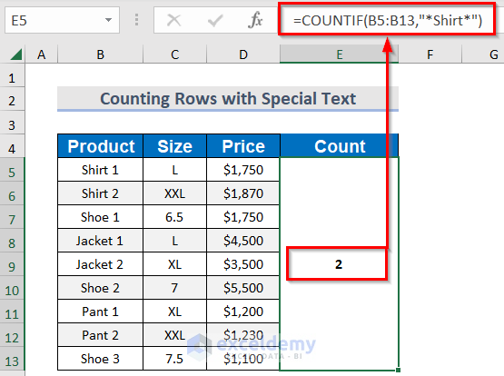
=COUNTIF(B5:B13,"*Shirt*")B5:B13 is the range, and between the wildcards, Shirt is used for searching this text.
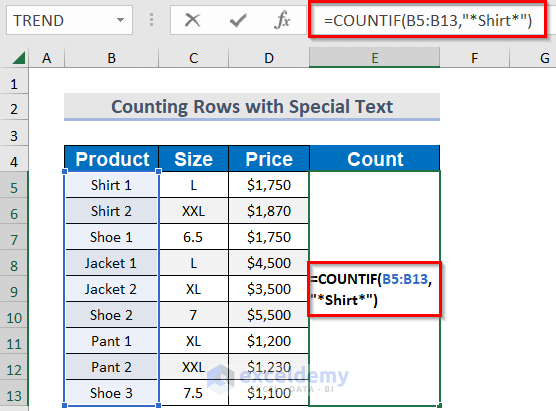
➤ Press ENTER.
➤ It will show the number of shirts in the Product column.
Method-3 – Combination of Functions to Count Rows Based on Multiple Criteria
Steps:
➤ Select the output cell in the Count column.
➤ Type the following function here:
=SUMPRODUCT(--(ISNUMBER(FIND("Shirt",B5:B13))+ISNUMBER(FIND("Shoe",B5:B13))>0))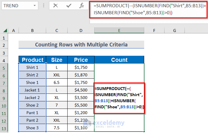
Formula Breakdown
B5:B13 is the range. Then, using the FIND function, you will find the desired texts Shirt and Shoe.
The ISNUMBER function will return an array containing 1 and 0. 1 will be for the case where the criteria are met, and 0 is for not meeting the criteria.
The SUMPRODUCT function will add up the values.
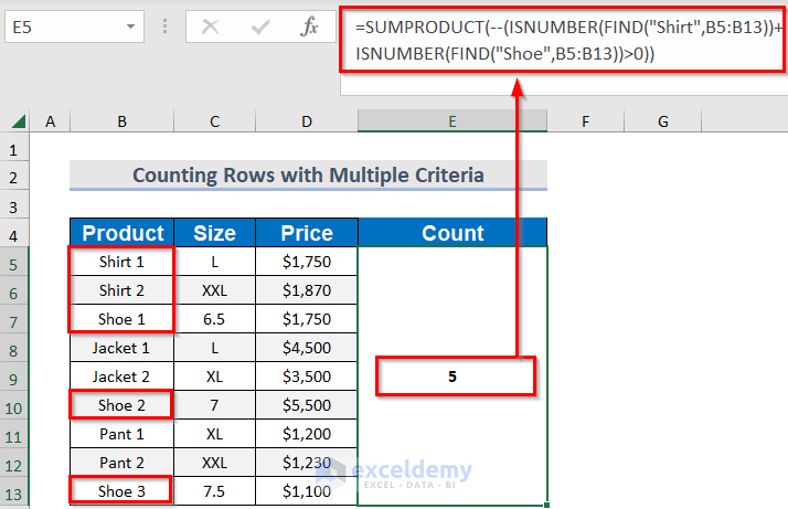
➤ Press ENTER.
➤ It will show up the number of shirts and shoes in the Product column.
Method-4 – Counting Rows with Non-Text Values
Steps:
➤ Select the output cell in the Count column.
➤ Type the following function here:
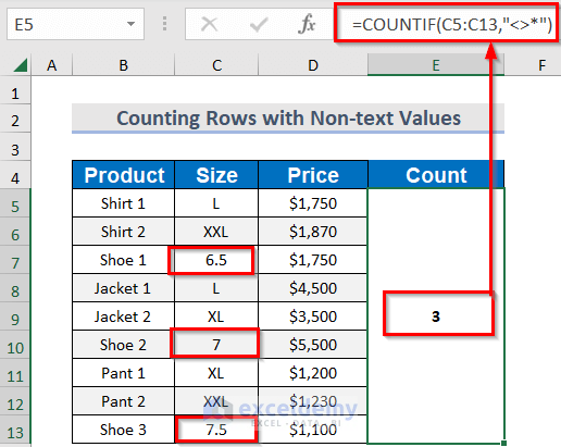
=COUNTIF(C5:C13,"<>*")C5:C13 is the range, and before the wildcard, <> is used, which means Not Equal to.
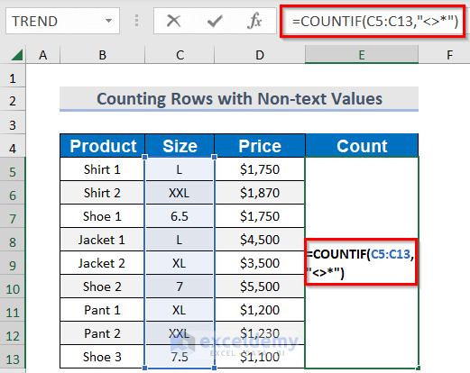
➤ Press ENTER.
➤ It will show up the number of numerical values in the Size column.
Method-5 – Applying SUMPRODUCT & ISTEXT Functions
Steps:
➤ Select the output cell in the Count column.
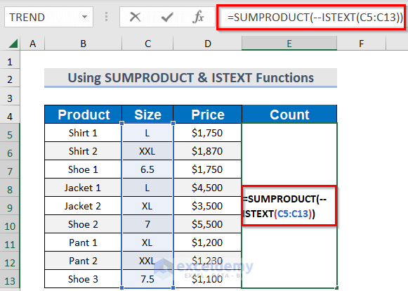
➤ Type the following function here:
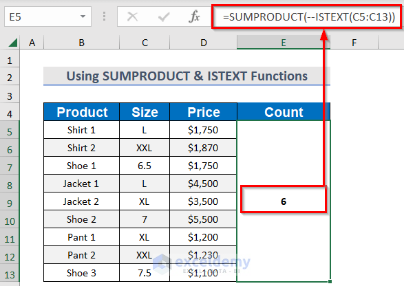
=SUMPRODUCT(--ISTEXT(C5:C13))C5:C13 is the range, the ISTEXT function will check out if there are texts and then will return TRUE and if there are no texts then it will return FALSE. Then — will convert TRUE into 1 and FALSE into 0. The SUMPRODUCT function will sum up the values.
➤ Press ENTER.
➤It will show up the number of texts in the Size column.
Method-6 – Use of SUM, IF & ISTEXT Functions to Count Rows with Text
Steps:
➤ Select the output cell in the Count column.
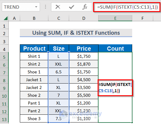
➤ Type the following function here.
=SUM(IF(ISTEXT(C5:C13),1))C5:C13 is the range, the IF function will return 1 if there is text and then the SUM function will sum up these values.
➤ Press ENTER.
➤It will show up the number of texts in the Size column.
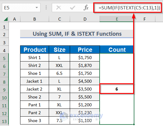
If you use an Excel version other than Excel 365, you may need to press CTRL+SHIFT+ENTER.
Method-7 – Counting Rows with Filtered Texts
Following this method, you can count the visible values only after filtering. Before filtering data, you must do extra tasks like the one below.
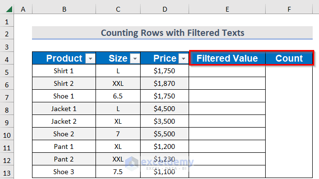
Steps:
➤Select cell E5 of the Filtered Value column.
➤ Type the following formula:
=SUBTOTAL(103,C5)To identify all hidden cells, filtered out and hidden manually, function_num is used as 103. And C5 is the reference.
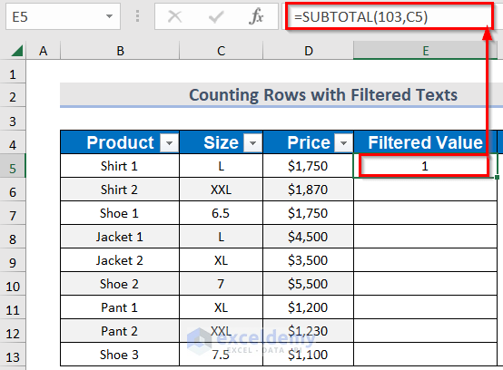
➤ Press ENTER.
➤Drag down the Fill handle tool.
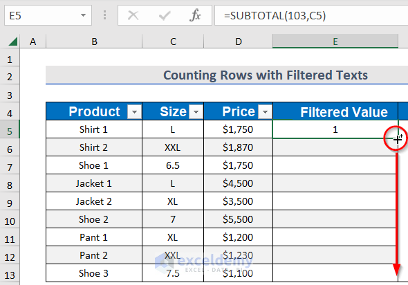
You will get 1 for all of the rows.
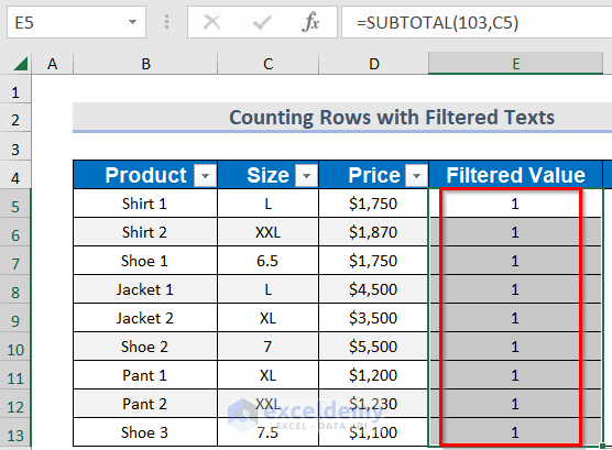
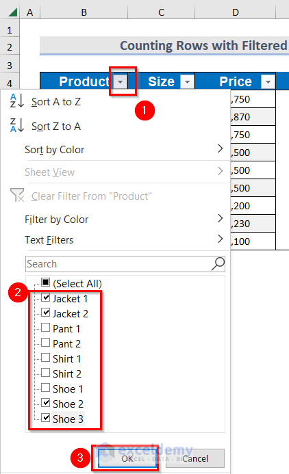
➤ You can filter the values according to your needs.
➤ Select the output cell in the Count column.
➤ Type the following formula:
=COUNTIFS(C5:C13, "*", E5:E13, 1)To count the number of visible texts, you can use the COUNTIFS function.
➤ Ppress ENTER.
➤ It will return the number of texts visible in the Size column.
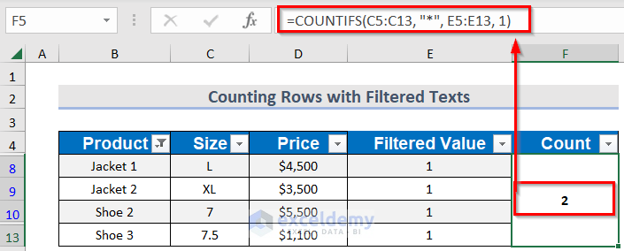
You can do the aforementioned task by typing only the following formula.
=SUMPRODUCT(SUBTOTAL(103, INDIRECT("C"&ROW(C5:C13))), --(ISTEXT(C5:C13)))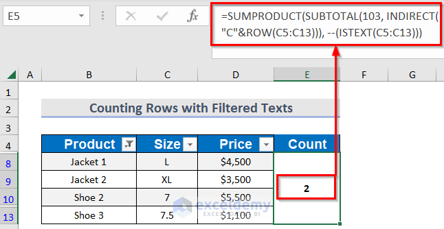
Use the following formula.
=SUMPRODUCT(SUBTOTAL(103, OFFSET(C5:C13, ROW(C5:C13) - MIN(ROW(C5:C13)),,1)), -- (ISTEXT(C5:C13)))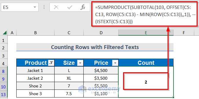
The following steps, you can change the filtered text.
- Click on the drop-down arrow >> then from the list >> select required texts >> press OK.
Download Practice Workbook
<< Go Back to Count Rows | Formula List | Learn Excel
Get FREE Advanced Excel Exercises with Solutions!

