Method 1 – Determining Average Price
Steps:
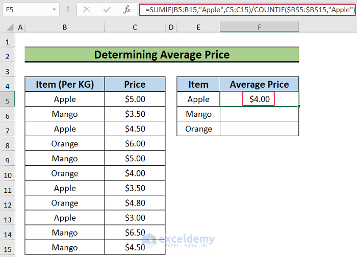
- Select the F5 cell and write down the following formula,
=SUMIF(B5:B15,"Apple",C5:C15)/COUNTIF($B$5:$B$15,"Apple")- Hit Enter.
- We will get the average price of the item.

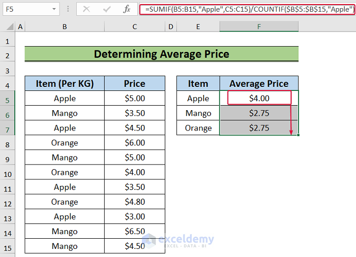
- Lower the cursor down to AutoFill the rest of the cells.

Formula Breakdown:
- SUMIF(B5:B15,”Apple”,C5:C15): The SUMIF function will go through the B5:B15 range and look from “Apple”. It will sum all the prices associated with “Apple” in the range C5:C15.In this case the summation will be 16.
- COUNTIF($B$5:$B$15,”Apple”): The COUNTIF function will scan through the cells in the range B5:B15 and return the number of occurrence of “Apple” in that cell range. It will be 4.
- SUMIF(B5:B15,”Apple”,C5:C15)/COUNTIF($B$5:$B$15,”Apple”): This one is simply the formula of average price. We have the total number of apples over the total price of the apples. In this instance, it will be $16 by 4 or $4.
Method 2 – Using COUNTIF and SUMIF with Condition
Steps:
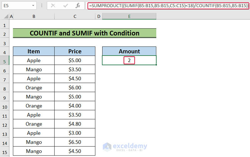
- Begin with, select the E5 cell and write the following formula down.
=SUMPRODUCT((SUMIF(B5:B15,B5:B15,C5:C15)<18)/COUNTIF(B5:B15,B5:B15))- Hit the Enter button.
- We will get the number of items that have a total price of less than $18.

Formula Breakdown:
- COUNTIF(B5:B15,B5:B15): This will return an array of values. The COUNTIF function will look for the number of occurrence of “Apple”, “Mango” and “Orange” as it moves from cell B5 to B15 and for each value in each cell it will look for number of occurrences of that value in the B5:B15 range and return the number. The result would be something like this : {4;4;4;3;4;3;4;3;4;4;4}.
- SUMIF(B5:B15,B5:B15,C5:C15)<18): At first, the SUMIF function will look for “Apple”, “Mango” and “Orange” in each cell. In the C5 cell, it will have Apple. So it will sum all the prices of Apple from the C5:C15 range and return $16. Then. it will sum for Mango and return $19.5 and then again it will sum for Apple and return $16 and it will do the same as it move from B5 to B15 and finally return an array like this : {16;19.5;16;14.8;19.5;14.8;16;14.8;16;19.5;19.5}. It will evaluate the values if they are less than $18 or not. Then it will return an array of True and False like this: {True;False;True;True;False;True;True;True;True;False;False}.
- SUMPRODUCT((SUMIF(B5:B15,B5:B15,C5:C15)<18)/COUNTIF(B5:B15,B5:B15)):The True values will be replaced by 1 and the False values with 0. These array with 1’s and 0’s will be divided by the array returned by the COUNTIF function and will return an array like this: {0.25;0;0.25;0.333333;0;0.333333;0.25;0.333333;0.25;0;0}. Finally, the SUMPRODUCT function will sum these values and will return 2.
Download Practice Workbook
You can download the practice workbook here.
Related Articles
- How to Use Nested COUNTIF Function in Excel
- How to Use COUNTIF and COUNTA Functions Together in Excel
- How to Use IF and COUNTIF Functions Together in Excel.
<< Go Back to Excel COUNTIF Function | Excel Functions | Learn Excel
Get FREE Advanced Excel Exercises with Solutions!


How could you perform the same count of records with SUMPRODUCT((SUMIFS)/(COUNTIF)? Trying count how many sumifs records (not sum value) with two criteria vs one. The return I am looking for is of the total sum value using a range (>0 & <10000), count how many excel finds to total the sum value produced.
Hello BRIAN,
Thanks for your comment. You can apply two criteria by using the SUMIF function twice in the formula. The formula is:
=SUMPRODUCT((SUMIF(B5:B15,B5:B15,C5:C15)<10000)*(SUMIF(B5:B15,B5:B15,C5:C15)>0)/COUNTIF(B5:B15,B5:B15))This will count the number of products whose total sum value is greater than 0 and less than 10000.
Regards
Mahfuza Anika Era
ExcelDemy